Modified KNN-LVQ for Stairs Down Detection Based on Digital Image
on
LONTAR KOMPUTER VOL. 12, NO. 3 DECEMBER 2021
DOI : 10.24843/LKJITI.2021.v12.i03.p02
Accredited Sinta 2 by RISTEKDIKTI Decree No. 30/E/KPT/2018
p-ISSN 2088-1541
e-ISSN 2541-5832
Modified KNN-LVQ for Stairs Down Detection Based on Digital Image
Ahmad Wali Satria Bahari Johana1, Sekar Widyasari Putrib2, Granita Hajarc3, Ardian Yusuf Wicaksonoa4
aInformatics, Faculty of Information Technology and Industry, Institut Teknologi Telkom Surabaya
Surabaya, Indonesia
1ahmadsatria13@ittelkom-sby.ac.id(Corresponding author)
bDigital Business, Faculty of Information Technology and Industry, Institut Teknologi Telkom Surabaya
Surabaya, Indonesia
cLogistics Engineering, Faculty of Information Technology and Industry, Institut Teknologi Telkom Surabaya
Surabaya, Indonesia
Abstract
Persons with visual impairments need a tool that can detect obstacles around them. The obstacles that exist can endanger their activities. The obstacle that is quite dangerous for the visually impaired is the stairs down. The stairs down can cause accidents for blind people if they are not aware of their existence. Therefore we need a system that can identify the presence of stairs down. This study uses digital image processing technology in recognizing the stairs down. Digital images are used as input objects which will be extracted using the Gray Level Co-occurrence Matrix method and then classified using the KNN-LVQ hybrid method. The proposed algorithm is tested to determine the accuracy and computational speed obtained. Hybrid KNN-LVQ gets an accuracy of 95%. While the average computing speed obtained is 0.07248 (s).
Keywords:Visual Impairments, GLCM, KNN, LVQ, Digital Image
Disability is a condition where a person has limitations in his physical condition. One type of disability is blindness, which is someone who has limited vision. They need tools to facilitate their activities. In this case, blind people often use sticks to detect objects around them and help them move. However, the stick itself has a weakness, where blind people have difficulty recognizing the types of objects around them. The ability to identify obstacles is also necessary for blind people. Where several obstacles can endanger their safety. Therefore, blind people need technology that can help them detect obstacles around them. One such obstacle is the down of the stairs. Where the stairs down is quite dangerous for anyone who falls.
Over the past few years, several technologies have been developed to help the visually impaired in their movements. Ultrasonic sensors have often been used to provide navigation or object detection. The research by Arnesh Sen Kaustav Sen Jayoti Das has developed a system to avoid an obstacle by using ultrasonic sensors. The ultrasonic sensors are paired up on the chest, knee, and toe[1]. However, that technique has limitations, where the sensor cannot detect objects that cannot be touched, such as stairs down. Because the sensor emits ultrasonic waves in a straight line and requires many sensors that attach to the body to detect obstacles, some technologies
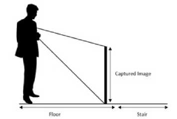
Figure 1. Camera Position
are being developed to help blind people currently based on an image to identify the obstacle. That has done by Alessandro Grassi by using a single smartphone camera. In that research, the system can identify obstacles such as traffic lights and doors[2]. Fitri Utaminingrum develops a wheelchair that able to detect stairs down by using a camera. That research uses GLCM and LVQ for the algorithm to classify between stairs down and floor. Fitri Utaminingrum develops a wheelchair that can detect stairs down by using a camera. That research uses GLCM and LVQ for the algorithm to classify between stairs down, and floor [3].
Several studies described illustrate that some technologies can help blind people in carrying out their activities. In this study, we use digital image processing technology to detect stairs down. This study uses Gray Level Co-occurrence Matrix feature extraction to calculate the feature values of the input image. The classification method that we propose is a hybrid K nearest neighbor algorithm and Learning vector quantization. KNN can find the closest distance between testing data and training data. Learning vector quantization has advantages in terms of computational speed. Learning vector quantization can carry out the training and testing process quickly, where fast computing time is very influential in the comfort of blind people.
The source of this research dataset was taken from several different buildings. Each building has the characteristics of stairs with different ceramics. Some buildings have the characteristics of stairs with large tiled floors, which have a unique value that is different from small tile floors. A camera is placed on the chest, as shown in Fig 1. Two classes are used to detect stairs down. The two classes are stairs down and floors. The image taken from the camera is 480x640 pixels. In the picture, ROI will be taken as an indicator of the stairs down or floor. The ROI taken is 400x150 pixels and is at the bottom of the image. ROI image that is used during the training process is taken manually. Researchers take ROI, which has characteristics as stairs down, and ROI, which has floor characteristics. For taking ROI training, there is no provision for coordinates, but the size taken is 400x150. Meanwhile, when the testing process, ROI is taken automatically, the coordinate position used is fixed. The coordinates of the test ROI are at coordinates (40,400) to (440,550). Figure 2 shows the position of the ROI taken during testing. Figure 3(a) shows the ROI of the stairs, and Figure 3(b) shows the ROI of the floors. In this research, the data source used is divided into 2. The data source consists of images used during the training process (200 images) and a set of images used during the testing process (40 images).
Gray Level Co-occurrence Matrix (GLCM) is a method that is often used in conducting texture analysis or feature extraction[4][5]. GLCM analyzes a pixel in a digital image and determines the level of gray that occurs. The image to be performed feature extraction using Gray Level Cooccurrence matrix must be converted into a grayscale image. Gray Level Co-Occurrence Matrix has two parameters, namely distance, and angle. Characteristics obtained from the matrix pixel
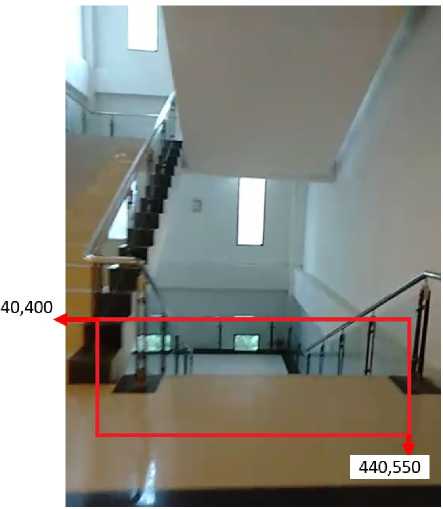
Figure 2. Input Image
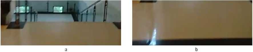
Figure 3. (a) ROI of Stairs down (b) ROI of Floor
values, which have a certain value and form a pattern angle [6][7][8]. The angles in GLCM are θ = 0o, 45o, 90o, and 135o and the distance values are d=1, 2, 3, and 4. Figure 4 is the angular orientation on GLCM. GLCM carries out several stages to perform feature extraction. The first stage is to form the initial GLCM matrix from a pair of 2 pixels based on a predetermined angle and distance. Then form a symmetric matrix by adding the GLCM matrix with the transpose matrix. Then normalize the GLCM matrix by dividing each matrix element by the number of pixel pairs. Six features will be generated from the GLCM feature extraction process. The following are six features used in this study[9]:
-
1. Contrast: This feature calculates the difference in the gray level of an image. The high or low contrast value depends on the amount of difference in the gray level in the image. The contrast value is obtained by equation 1.
L
Contrast = ^ (a — b)2 a,b=0
(1)
-
2. Homogeneity: This feature calculates the value of gray homogeneity in an image. The homogeneity value will be higher if the gray level is almost the same. The homogeneity values are obtained by equation 2.
Homogeneity =
L
X
a,b=0
(a, b)x2
1|a — b|
(2)
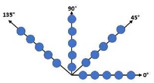
Figure 4. Angle Orientation
-
3. Correlation: This feature shows how the pixel reference correlates with its neighbors. The correlation values are obtained by equation 3.
Correlation = XX Pi,j (a - ^ - ^) (3)
a,b=0
-
4. EEnergy: This feature calculates the level of gray distribution in an image. The energy values are obtained by equation 4.
L
Energy = ∑ P2(α,b) (4)
a,b=0
-
5. Dissimilarity: The dissimilarity values are obtained by equation 5.
L
Dissimilarity = Pa,b|a - b| (5)
a,b=0
-
6. AAngular Second Moment: The Angular second moment values are obtained by equation 6.
L
ASM = X P(i,j)2 (6)
a,b=0
where :
-
• L = Number of gray levels in the image as specified by Number of levels
-
• a,b = Pixel coordinate
-
• P = Element a,b of the normalized symmetrical GLCM
-
• ϑ = the GLCM mean (being an estimate of the intensity of all pixels in the relationships that contributed to the GLCM)
-
• σ2 = the variance of the intensities of all reference pixels in the relationships that contributed to the GLCM
K nearest neighbor (KNN) is a supervised learning algorithm, in which this algorithm generates a classification based on the majority of the k-value categories provided in the training data [10] [11]. The purpose of this algorithm is to classify new objects based on attributes and samples from training data. The K Nearest neighbor algorithm uses neighborhood classification as the predicted value for the new instance value.[12]. Training data is placed in a place that will be used during the classification process. The unknown sample class is determined by a majority vote of
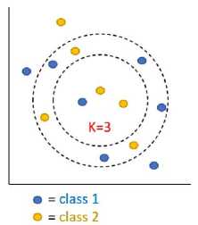
Figure 5. KNN concept
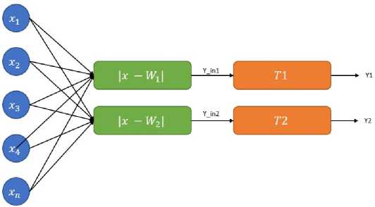
Figure 6. LVQ Architecture
its neighboring samples in the training pattern space [13][14]. The most influential parameter on K nearest neighbor is the k-value. Where k-value is a parameter of how many nearest neighbors of the object are classified. Figure 5 is an example of the KNN concept. Where the k-value used is 3. Then the algorithm will find the three closest neighbors using the Euclidian distance equation. Equation 7 is a way to find the nearest neighbor using Euclidian distances. After getting the three closest neighbors, the next step is to calculate the majority of the class in the three neighbors. Where the majority class will be selected as the result of the classification.
D(a,b)
n
X(ak - bk)2
k=1
(7)
Where :
-
• n = number of data
-
• D(a, b) = closest euclidean distance
-
• a = data 1
-
• b = data 2
-
• k = feature to - n
Learning Vector Quantization (LVQ) is part of the classification of artificial neural networks with supervised competitive learning [15]. LVQ works by using a clustering method where the tar-get/class has been defined by the architecture [16]. The LVQ learning model is trained significantly faster than other algorithms such as Back Propagation Neural Network. It can summarize
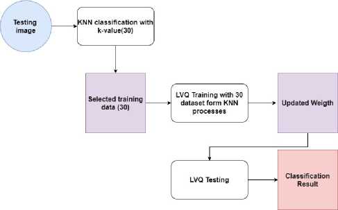
Figure 7. Hybrid KNN-LVQ
or reduce large datasets to a small number of vectors. The competitive layer will automatically learn to classify the input vectors. The classes obtained from this competitive layer only depend on the distance between the input vectors. If the input vectors are close to the same, the competitive layer will classify the two input vectors into the same class [17][18]. Figure 6 is an LVQ architecture with two classes. The following are some of the steps in running LVQ [19]:
-
1. Initialization of initial weight (Wj) and value of learning rate (α). The weights used are equal to the number of classes. Where each weight represents its respective class.
-
2. Determine the number of training iterations
-
3. Find the closest distance (j) using equation 8.
-
4. Update the selected weight value as the minimum value. If the selected condition is the same as the target, an update is carried out using equation 9. If the selected weight is not the same as the target, then the update uses equation 10.
Wj = Wj (old) + α(x — Wj (old))(9)
Wj = Wj (old) — α(x — Wj (old))(10)
-
5. Stop the training process until the specified number of iterations
Where :
-
• Wj = Weight of LVQ
-
• Wj (old) = Old weight
-
• j = Distance value
-
• x = Training data
-
• α = Learning rate
The limitation of the KNN classifier is a false classification of test images when the majority of the nearest neighbors have closely matched features[20]. The computational time of KNN depends on the amount of training data used. The more training data, the longer it takes. To overcome this problem, KNN could be combined with another classifier[21][22]. Here we combine KNN with
LONTAR KOMPUTER VOL. 12, NO. 3 DECEMBER 2021 DOI : 10.24843/LKJITI.2021.v12.i03.p02
Accredited Sinta 2 by RISTEKDIKTI Decree No. 30/E/KPT/2018
LVQ to classifying between floor and stairs down. Where LVQ has the advantage of speeding up the training and testing process. The idea is that the program runs KNN to get 30 data from 200 training data that has the closest value to the test data so that there are only 30 selected training data to be continued in the LVQ process. Where training is carried out on the LVQ to update the initial weight. The initial weight used before training is the average value of the GLCM features of each class. Two weights represent the class of stairs down and floor. The LVQ training process was carried out 100 times. After the training process is complete, it is continued to test data testing with LVQ using the latest weights from the training process. The KNN-LVQ hybrid concept is depicted in figure 7.
There are 240 pieces of image data used in this study. Where the image will be used for training data and partly used as test data. Training and testing data use different images. In the training process using the KNN-LVQ hybrid algorithm, there are as many as 200 images consisting of images indicating the stairs down and images indicating the floor. In the testing process, 40 images consist of images of stairs down and floors. In the testing process to be carried out, we look for the accuracy value obtained using equation 11 [23].TP (true positive) shows the appropriate prediction results, namely the stairs down. TN (true negative) indicates an incorrect prediction result. Where the test data is the stairs down, but the results of the floor prediction. FP (false positive) indicates the correct prediction result, namely the floor. FN (false negative) indicates an incorrect prediction result. Where the test data is the floor, but the prediction results are stairs down.
A =
TP + TN
TP + FP + TN + FN
(11)
Where :
-
• A = Accuracy
-
• T P = True positive
-
• T N = True negative
-
• F P = False positive
-
• F N = False negative
Testing is carried out by comparing the accuracy results obtained from 3 classification methods. The first method is K nearest neighbor, then Learning Vector Quantization. Next is our proposed method, namely Hybrid KNN-LVQ. This test is carried out with the same parameters. The GLCM distance and angle parameters used are d =1 and θ = 0o. The GLCM parameter is used when performing feature extraction. So that this test is carried out with the same test data and the same feature value. As for LVQ, the training iterations carried out were 100 times and the learning rate used was α = 0.5. Iteration and learning rate parameters are used during the LVQ and Hybrid KNN-LVQ classification processes. Tests were carried out using 40 data consisting of 20 data features of stairs down and 20-floor feature data. This test is shown in Table 1. From the tests’ results, the K nearest neighbor algorithm gets the lowest accuracy, which is 90%. The Learning Vector Quantization Algorithm gets an accuracy of 92.5%. While the method that we propose can get a better accuracy result that is 95%. These results indicate that the classification process carried out by Learning Vector Quantization gets better results when the training data is selected using K Nearest Neighbor. By using the process of finding the nearest neighbor on K nearest neighbor, we can obtain a dataset for training that is more in line with the given testing data.
|
Method |
Stairs down |
Floor |
Accuracy |
|
LVQ |
18 |
19 |
92.5% |
|
KNN |
18 |
18 |
90% |
|
Hybrid KNN-LVQ |
19 |
19 |
95% |
Table 2. Result of Computation Time Testing
|
No |
LVQ |
KNN |
Hybrid LVQ-KNN |
|
1 |
0.02600 (s) |
0.02499 (s) |
0.06601 (s) |
|
2 |
0.02899 (s) |
0.06100 (s) |
0.07702 (s) |
|
3 |
0.02599 (s) |
0.05937 (s) |
0.04302 (s) |
|
4 |
0.03001 (s) |
0.10656 (s) |
0.11347 (s) |
|
5 |
0.03000 (s) |
0.02700 (s) |
0.08907 (s) |
|
6 |
0.02600 (s) |
0.05902 (s) |
0.05480 (s) |
|
7 |
0.02900 (s) |
0.03400 (s) |
0.08600 (s) |
|
8 |
0.02500 (s) |
0.03100 (s) |
0.08454 (s) |
|
9 |
0.03200 (s) |
0.02600 (s) |
0.06385 (s) |
|
10 |
0.02500 (s) |
0.05001 (s) |
0.04700 (s) |
|
Average |
0.02779 (s) |
0.04789 (s) |
0.07248 (s) |
Computational time testing is carried out to determine the average speed of each algorithm in classifying. This is quite influential on the comfort for users of the stair down detection system. It takes computing time as quickly as possible in the detection. This test uses ten pictures of the same stairs down. In table 2, it can be seen that LVQ produces the fastest computation time of 0.02779 (s). While the KNN-LVQ hybrid produces the slowest computation time, which is 0.07248 (s). This is because the KNN-LVQ hybrid performs two processes, namely the KNN process to obtain K-30 as training data for the training process and test on LVQ.
TThis research aims to create a system that can detect the presence of stairs down. The GLCM feature extraction method was used to generate six feature values. The six features are contrast, homogeneity, energy, angular second moment, correlation, and dissimilarity. We propose a combination of classification algorithms in determining the class on the test image, where there are two classes, namely stairs down and floors. The combined algorithms are K nearest neighbor and Learning vector quantization. We call this merger Hybrid KNN-LVQ, where KNN works to get K-30. K-30 is the 30 data that is closest in value to the test data. Furthermore, the LVQ process conducts training on 30 selected data to update the weights and the testing process on the test data. From the results of the tests conducted, the hybrid KNN-LVQ method produced a better accuracy of 95%. However, the KNN-LVQ method has a longer computation time than the comparison algorithm, as shown in Table 2.
References
-
[1] A. Sen, K. Sen, and J. Das, “Ultrasonic blind stick for completely blind people to avoid any kind of obstacles,” in 2018 IEEE SENSORS, 2018, pp. 1–4.
-
[2] A. Grassi and C. Guaragnella, “Defocussing estimation for obstacle detection on single camera smartphone assisted navigation for vision impaired people,” in 2014 IEEE International Symposium on Innovations in Intelligent Systems and Applications (INISTA) Proceedings, 2014, pp. 309–312.
-
[3] A. W. S. Bahari Johan, F. Utaminingrum, and T. K. Shih, “Stairs descent identification for smart wheelchair by using glcm and learning vector quantization,” in 2019 Twelfth International Conference on Ubi-Media Computing (Ubi-Media), 2019, pp. 64–68.
-
[4] R. Yusof and N. R. Rosli, “Tropical wood species recognition system based on gabor filter as image multiplier,” in 2013 International Conference on Signal-Image Technology InternetBased Systems, 2013, pp. 737–743.
-
[5] C. Malegori, L. Franzetti, R. Guidetti, E. Casiraghi, and R. Rossi, “Glcm, an image analysis technique for early detection of biofilm,” Journal of Food Engineering, vol. 185, pp. 48–55, 2016.
-
[6] M. Saleck, A. ElMoutaouakkil, and M. Moucouf, “Tumor detection in mammography images using fuzzy c-means and glcm texture features,” in 2017 14th International Conference on Computer Graphics, Imaging and Visualization (CGiV). Los Alamitos, CA, USA: IEEE Computer Society, may 2017, pp. 122–125.
-
[7] Z. khan and S. Alotaibi, “Computerised segmentation of medical images using neural networks and glcm,” in 2019 International Conference on Advances in the Emerging Computing Technologies (AECT). Los Alamitos, CA, USA: IEEE Computer Society, feb 2020, pp. 1–5.
-
[8] S. Barburiceanu, R. Terebes, and S. Meza, “3d texture feature extraction and classification using glcm and lbp-based descriptors,” Applied Sciences, vol. 11, no. 5, 2021. [Online]. Available: https://www.mdpi.com/2076-3417/11/5/2332
-
[9] T. S. A. Sukiman, M. Zarlis, and S. Suwilo, “Feature extraction method glcm and lvq in digital image-based face recognition,” Applied Sciences, vol. 4, no. 1, 2019.
-
[10] M. Kenyhercz and N. Passalacqua, “Chapter 9 - missing data imputation methods and their performance with biodistance analyses,” in Biological Distance Analysis, M. A. Pilloud and J. T. Hefner, Eds. San Diego: Academic Press, 2016, pp. 181–194.
-
[11] “Chapter 9 - object categorization using adaptive graph-based semi-supervised learning,” in Handbook of Neural Computation, P. Samui, S. Sekhar, and V. E. Balas, Eds. Academic Press, 2017, pp. 167–179.
-
[12] K. Taunk, S. De, S. Verma, and A. Swetapadma, “A brief review of nearest neighbor algorithm for learning and classification,” in 2019 International Conference on Intelligent Computing and Control Systems (ICCS), 2019, pp. 1255–1260.
-
[13] X. Zhu and T. Sugawara, “Meta-reward model based on trajectory data with k-nearest neighbors method,” in 2020 International Joint Conference on Neural Networks (IJCNN), 2020, pp. 1–8.
-
[14] A. K. Gupta, “Time portability evaluation of rcnn technique of od object detection — machine learning (artificial intelligence),” in 2017 International Conference on Energy, Communication, Data Analytics and Soft Computing (ICECDS), 2017, pp. 3127–3133.
-
[15] P. Melin, J. Amezcua, F. Valdez, and O. Castillo, “A new neural network model based on the lvq algorithm for multi-class classification of arrhythmias,” Information Sciences, vol. 279, pp. 483–497, 2014.
-
[16] S. Qiu, L. Gao, and J. Wang, “Classification and regression of elm, lvq and svm for e-nose data of strawberry juice,” Journal of Food Engineering, vol. 144, pp. 77–85, 2015.
-
[17] E. Subiyantoro, A. Ashari, and Suprapto, “Cognitive classification based on revised bloom’s taxonomy using learning vector quantization,” in 2020 International Conference on Computer Engineering, Network, and Intelligent Multimedia (CENIM), 2020, pp. 349–353.
-
[18] I. M. A. S. Widiatmika, I. N. Piarsa, and A. F. Syafiandini, “Recognition of the baby footprint characteristics using wavelet method and k-nearest neighbor (k-NN),” Lontar Komputer : Jurnal Ilmiah Teknologi Informasi, vol. 12, no. 1, p. 41, mar 2021. [Online]. Available: https://doi.org/10.24843%2Flkjiti.2021.v12.i01.p05
-
[19] K. J. Devi, G. B. Moulika, K. Sravanthi, and K. M. Kumar, “Prediction of medicines using lvq methodology,” in 2017 International Conference on Energy, Communication, Data Analytics and Soft Computing (ICECDS), 2017, pp. 388–391.
-
[20] E. Haerani, L. Apriyanti, and L. K. Wardhani, “Application of unsupervised k nearest neighbor (UNN) and learning vector quantization (LVQ) methods in predicting rupiah to dollar,” in 2016 4th International Conference on Cyber and IT Service Management. IEEE, apr 2016.
-
[21] O. R. de Lautour and P. Omenzetter, “Nearest neighbor and learning vector quantization classification for damage detection using time series analysis,” Structural Control and Health Monitoring, 2009.
-
[22] P. Sonar, U. Bhosle, and C. Choudhury, “Mammography classification using modified hybrid svm-knn,” in 2017 International Conference on Signal Processing and Communication (ICSPC), 2017, pp. 305–311.
-
[23] R. J. A. Kautsar, F. Utaminingrum, and A. S. Budi, “Helmet monitoring system using hough circle and HOG based on KNN,” Lontar Komputer : Jurnal Ilmiah Teknologi Informasi, vol. 12, no. 1, p. 13, mar 2021.
150
Discussion and feedback