Frequency Band and PCA Feature Comparison for EEG Signal Classification
on
LONTAR KOMPUTER VOL. 12, NO. 1 APRIL 2021
DOI : 10.24843/LKJITI.2021.v12.i01.p01
Accredited Sinta 2 by RISTEKDIKTI Decree No. 30/E/KPT/2018
p-ISSN 2088-1541
e-ISSN 2541-5832
Frequency Band and PCA Feature Comparison for EEG Signal Classification
I Wayan Pio Pratamaa1, Made Windu Antara Kesimana2, I Gede Aris Gunadib3
aGanesha University of Education, Computer Science Departement
Denpasar, Indonesia
2antara.kesiman@undiksha.ac.id
Abstract
The frequency band method is popular in signal processing; this method separates EEG signals into five bands of frequency. Besides the frequency band, the recent research show PCA method gives a good result to classify digits number from EEG signal. Even PCA give a good accuracy to classify digit number from EEG signal, but there are no research shows which one yielded better accuracy between PCA and frequency band to classify digit number from EEG signals. This paper presents the comparison between those methods using secondary data from MindBigData (MDB). The result shows that the frequency band and PCA achieve 9% and 12,5% on average accuracy with the EPOC dataset. The paired Wilcoxon test produces a significant difference in accuracy between methods in the digit classification problem. Experiment with Muse dataset provides 31% accuracy with frequency band method and 24,8% with PCA method. The result is competitive compared to other experiments to classify digit numbers from EEG signals. In conclusion, there is no winner between the two methods since no method fits both datasets used in this research.
Keywords: Digit Classification, Feature Comparison, Frequency Band, PCA, EEG Signal, Wilcoxon Test
Digital signal processing (DSP) is a complex task yet a very hot topic for the researcher. One of the most popular topics in DSP is how to classify signals to be a piece of meaningful information. Voice recognition is one example of how DSP could lead this world to a phase that never happens before. Someone with their phone can give a command to send a message just by a voice, or someone could just turn on and off their car just by a hand clap. Something that feels impossible in the past now becomes a reality. Something even more surprising is brainwaves. Recently the use of brainwaves is increasingly widespread, ranging from detecting brain disease to moving robot hands. One of the most interesting is the use of brain waves to control computer screens or interfacing them. These waves are formed due to the interaction of the neurons in the brain. This interaction generates electricity and is known as brainwaves [1]. To get this signal researcher needs to use a device called electroencephalography. EEG is defined as a measurement of electrical activity produced by the brain [2]. The concept of interfacing a computer directly to the brain is a relatively new one, but the analysis of brain waves has been reported since 1929 [3]. Nowadays, controlling devices by the mind is a very controversial topic but highly researched. Some devices such as smartphones, laptops, and tablets, and even televisions to be used by people with disabilities, for which these technologies could be the only way of communication with the external environment. A BCI is defined as a device that measures the activity of the brain or central nervous system and converts these signals into artificial output [4]. A wide range of applications can apply knowledge of the EEG signal [5], but BCI is not an easy task. BCI research requires expertise and knowledge in many different fields such as signal processing, computer science, computational neuroscience, and embedded intelligent systems.
With the extraordinary benefits that can be obtained from EEG signals, many researchers are finally competing to apply EEG signals in many different applications. But unfortunately,
processing EEG signals so that they can be used in applications is not an easy thing to do. Apart from technical problems such as effective electrode placement and impedance between scalp, signal processing tasks are also difficult. One of the problems is the feature extraction method. Even a simple classifier, if we feed in high-quality data, can produce a high accuracy system. This reason made feature extraction becomes crucial in any classification problem.
Frequency band and PCA methods are widely used in the case of DSP and EEG signals specifically. The recent works related to EEG signals that using PCA to recognize digit numbers from EEG signals have been done in [6]. The researchers used data from MDB and collected it by a device called Insight with five channels and show that PCA based method yielded good accuracy, around 84%. Another research is using Multilayer Perceptron (MLP) to recognize digit numbers from EEG signals have been done in [2]. The data used in that experiment is from MindBigData (MDB) which is collected by a device called Muse with four channels. The research found the best accuracy is 27% with non boosted MLP. Another research is in ref. [7] which had tried to recognize digits numbers from EEG signals using CNN and yielded an accuracy of around 27-34%. The research also used data from MDB that collected by Muse device. Ref. [8] is another EEG research with power spectral density to detect pleasure and displeasure state with the highest accuracy result is 99,3%. However, there is no direct comparison between frequency band and PCA on an object of the problem with the same data and research environment. For this reason, this study conducted a comparison of both methods in a case to recognize digit numbers from the EEG signal. In the end, this research is expected to be a consideration in selecting the feature extraction method in the EEG signal problems so that it can be used in real applications such as BCI to detect a digit numbers signal.
This section will explain the stages carried out in the research. The general steps for classification research contain four major steps that are data acquisition, preprocessing, feature extraction, and testing. There is something to be noticed in that no specific training stage in this research. The reason behind this is that KNN is considered that called a lazy learner algorithm. The step that becomes the emphasis in this research is feature extraction using frequency band and PCA.
Fixed length EEG Signals, dimension (SGOCL 256)

Data Acquisition Download raw EEG signal Recording data in Jxtfile
Data Preprocessing
-
1. Sampling
-
2. Fixed length

Testing Method 10-fold validation is applied
70% training and 30% testing in 10 fold


For each fold 30% testing do : 1. Flattening 2. Predict normalization using training normalization 3. Predict PCA using traning PCA
KNN and compare average accuracy for both methods


For each fold 70% training do :
-
1. Flattening
-
2. Normalization
-
3. PCA is computed
For each fold 70% training and 30% testing do :
-
1. Frequency band is Computedfor each channels
-
2. Flattening
-
3. Normalization training
-
4 Predicttesting normalization using normalization training
The data that was used in this research is an EEG signal labeled with a digit of a number that can be found on the MDB website. There are four different datasets collected by four different devices on that website: Mindwave, EPOC, Insight, Muse. Some paper research such as [2], [6], and [7] had used this dataset for their research. That is a secondary dataset collected by another researcher. This research used the data collected by a device called EPOC as the main experiment and can be downloaded from the MDB website. The website provides data of the EEG signal in CSV format in a .txt file extension. This experiment used data that was measured by EPOC. The dataset contains 910,476 rows of data in total and labeled from -1 to 9. Label -1 stands for the subject with a random thought, and other labels thought of a digit number. The subject for this data collection is one with a healthy brain. EPOC has 14 channels, and each channel produces a CSV of decimal value as a result.
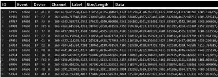
Figure 2. Data Snippet
File Format
Id
Event Device Channel
Code
Size
Data
-
: this is just for reference
-
: to differentiate between measurement event
-
: character to identify what device to use in the measurement
-
: a string to identify the 10/20 brain location of the signal
-
: label that the value can be 0, 1, 2, 3, 4, 5, 6, 7, 8, 9, -1.
-
: the size of the signal recorded
-
: amplitude as a result of the measurement
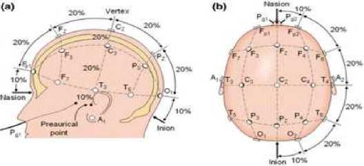
Only EPOC data follow the rule of 10/20 international electrode placement that is recommended [9]. One subject was stimulated by a digit of number from 0 to 9 in 2s and recorded by EPOC headset. Figure 3 shows in detail the standard of electrode placement. EPOC with 14 channels is qualified for this standard and be the reason that was used in this research. But at the end, this experiment, to get a fair comparison result with other research papers, also uses the Muse dataset from MBD. The experiment used all the data provided collected by Muse, which is 163932 in total. Both measurements by EPOC and Muse use the same subject and collected by the same researcher, and the only difference is the device and channel. More detail of the data can be found through this website http://www.mindbigdata.com/opendb/.
Considering the size of the data obtained, sampling was employed to make this research faster. For each label, 5600 rows of data were taken and 56,000 in total.
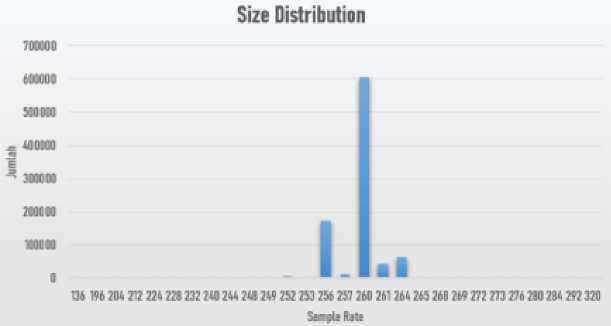
Figure 4. Data signal size/length distribution
Figure 4 explained that the majority signal length fell in 260. In theory, the EPOC sample rate is 128Hz [11]. So, to tackle this problem then the signal was padded with 0 or trimmed to make it had a fixed length of 256 values per 2s.
Since every 14 lines of data represent a measurement, then the data was flattened. Flattening is a process to convert the data into a 1-dimensional array for inputting it to the next layer [12]. This process would have made the dimension of the data was (400, 3584) after that min-max normalization was applied. Min-Max normalization is a method of normalization with performing linear transformations of the original data, thus resulting in a balance of values comparison between data before and after the process [13]. Equation 1 shows the min-max normalization formula,
normalized x =
(
'minRange + (x — minV alue)(maxRange - minRang e) . maxValue - minValue
)
(1)
Error! Reference source not found. is explained in detail step by step that needs to follow in this research. The thing to note is that normalization is carried out on the training data; for testing, data use predictor from training normalization.
Frequency is one of the most important criteria for assessing abnormalities in clinical EEGs and for understanding functional behaviors in cognitive research. There are five major brain waves distinguished by their different frequency ranges. These frequency bands from low to high frequencies, respectively, are typically categorized in specific bands such as 0.5-4 Hz (delta, δ), 4-8 Hz (theta, θ), 8-13 Hz (alpha, a), 13-30 Hz (beta, β) and >30 Hz (gamma, γ) [14]. i.e., alpha waves often appear in the eyes closed, waking state, and relaxed conditions, beta waves often arises when the person is thinking, theta waves in a range of 4–7 Hz and usually occurs when someone is in a night of light sleep, sleepy or stressed, delta waves in the range of 0.5–3 Hz and often present in the person in a state of deep sleep [15].
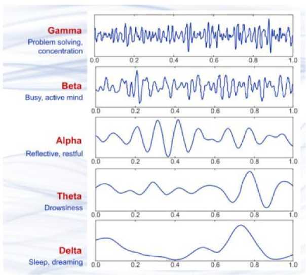
Figure 5. Four typical dominant brain normal rhythms [16].
FFT was employed to convert time domain signal to frequency. For each band, then power spectral, power ratio, and spectral entropy were calculated [17].
Power spectral,
[N(fk+1∕fs)]
PSIk= ∑ ∖Xl∖,k= 1,2.....k-1 (2)
i=[N(fk∕fs)]
Power ratio,
RIRj =
PSIi ∑⅛psιkj = 1,2.....k-1
(3)
Spectral entropy,
H =
-
1 log W
κ ∑ i=ι
RIRi log RIRi,j
1,2,
...,k
-1
(4)
Principal Component Analysis (PCA) is a technique to transforms several possibly correlated variables into a smaller number of variables called principal components [18]. PCA technique has many goals, including finding relationships between observations, extracting the most important information from the data, outlier detection and removal, and reducing the dimension of the data by keeping only the important information [19]. First, the covariance matrix of the data matrix (X) is calculated. Second, the eigenvalues and eigenvectors of the covariance matrix are calculated. In detail, to compute PCA can be seen in [20]. Figure 6 shown how PCA transformed data from a higher dimension to a lower dimension just by one component.
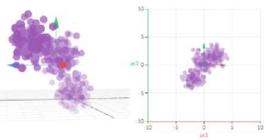
Figure 6. Illustration of PCA result [21]
The KNN algorithm completes its execution in two steps, first finding the number of nearest neighbors and second classifying the data point into a particular class using the first step. To find the neighbor, it makes use of distance metrics like euclidean distance, as given in equation 5 [22].
Distance =
√∑(*i -¾)
(5)
It chooses the nearest k samples from the training set, then takes the majority vote of their class where k should be an odd number to avoid ambiguity.
In testing, 10-fold validation was used. K-fold CV is a typical procedure to split the data randomly and evenly into K parts. The training set is built based on the K - 1 part of the dataset. The prediction accuracy of this candidate model is then evaluated on a test set containing the data in the hold-out part [23]. For each fold, accuracy is then calculated using equation 6.
TP + TN
(6)
accuracy = ——————— TP + TN + FP + FN
Where the term TP is truly positive, TN is a true negative, FP is false positive, and FN is false negative [24].
The experiment of this research reported the feature extraction and evaluation using 10-fold validation and accuracy metric.
To extract the frequency band feature, each channel in the data transformed into the frequency domain. FFT is the method that was used in this experiment.
Chsnntl :AF3 = CtiAnneIAFS

∣∣W FKlfHlV
■ UI Wn JSLSlRil -Uu MtVfcflI ∙∙ «ney MtIH-Uiiani ⅛1IM) IUI * AB: MIIZLIIMSaiH - MllZ »1295512 WS - MtΠφC SSASt-WMMi: 3MI2211.3-50:6IM.lt
Figure 7. FFT result
FFT produced a huge magnitude on zero frequency, so this was made the loss in detail. To solve this, a DC removal operation was then applied.
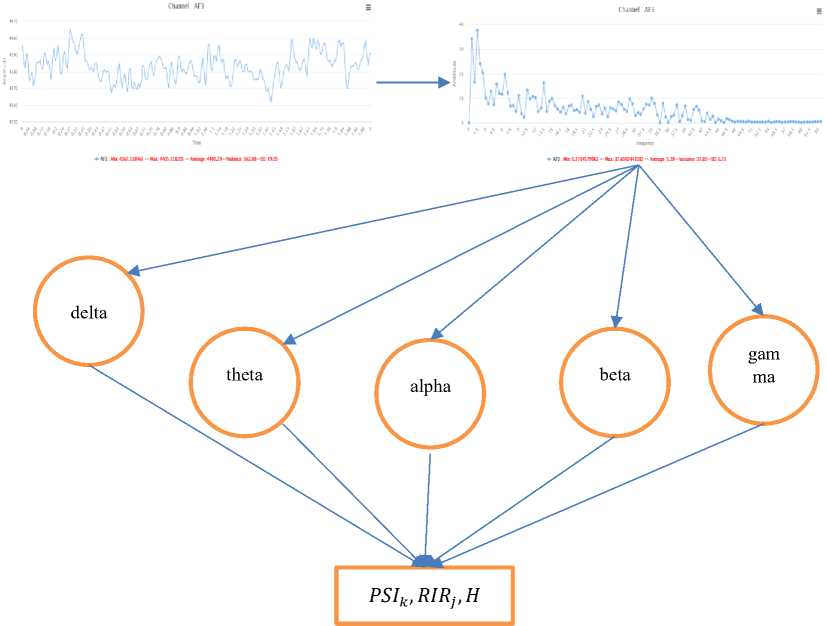
Figure 8. DC removal and frequency band applied
At the end of the flattening process, the dimension of the data became (400, 210). The flattening result then normalizes using equation (1) and ready to use in KNN classification.
To process the data with PCA, flattened and normalized were used to make each measurement unite and balance in weight. After that then PCA can be applied. PCA transforms original data into principal components. The principal component is the key factor when using PCA as a characteristic of a classification problem. Selecting the optimal principle will improve the chance to give a good experiment result. One of the important things to be considered is the cumulative variance explained. By making cumulative variance explained is as close as the original data will make optimal dimension and also keep the originality of the variance. To achieve this small experiment was conducted, and the result is drawn in Figure 9.
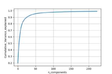
Figure 9. Cumulative variance explained
The graph explains to us that number component 186 will give 99% of the cumulative variance explained.
The first assessment was for the frequency band feature. KNN was employed with 210 features and 400 data in total. 70% of 400 data were used as training and 30% as testing with ten labels. Each label would have the same number of data in both training and testing. The Ten-fold validation method was also implemented to give a stable result, and the selected k was 3.
Table 1. Frequency band and KNN
|
Experiment |
Train Acc (%) |
Test Acc (%) |
|
1 |
40 |
9 |
|
2 |
39 |
11 |
|
3 |
39 |
8 |
|
4 |
42 |
9 |
|
5 |
46 |
8 |
|
6 |
40 |
7 |
|
7 |
41 |
7 |
|
8 |
46 |
7 |
|
9 |
39 |
12 |
|
10 |
38 |
12 |
The second experiment was the PCA. The same portion of data and parameters were used in this experiment.
Table 2. PCA and KNN
|
Experiment |
Train Acc (%) |
Test Acc (%) |
|
1 |
43 |
17 |
|
2 |
42 |
13 |
|
3 |
38 |
13 |
|
4 |
42 |
10 |
|
5 |
44 |
10 |
|
6 |
43 |
9 |
|
7 |
41 |
14 |
|
8 |
45 |
16 |
|
9 |
41 |
10 |
|
10 |
42 |
11 |
Clearly, from Table 1, the average accuracy for the frequency band with the KNN method is 41% for training and 9% for testing. On the other hand average accuracy for PCA with KNN are 42,1% for training and 12,3% for testing. Even clearly seen that average accuracy with PCA is better than frequency band in both training and testing set with a 10-fold validation method, a hypothesis test is still another consideration to believe this result significant based on the classic statistical method. Before the test is started normality of the result is tested using the Shapiro-Wilk test since the sample is less than 50. The result can be seen in Figure 10.
|
Kolmogorov-Smitnovi |
Statistic |
Shapiro-Wilk df |
Sig. | |||
|
Statistic |
df |
Sig. | ||||
|
TestAcc FrequencyBand |
.200 |
10 |
.2θθ' |
851 |
10 |
059 |
|
TestAcc PCA |
.198 |
10 |
.200’ |
909 |
10 |
.277 |
|
Train Acc Frequency Band |
236 |
10 |
.120 |
.818 |
10 |
024 |
|
Train Acc PCA |
183 |
10 |
2θθ' |
938 |
10 |
528 |
Figure 10. Normality Test
Since the sig. (p) ≥0,05, then the result is not normal. This condition didn't allow the use of a parametric statistical method. Wilcoxon test was used since both methods, as well as frequency band and PCA using the same data for training and testing.
|
N |
Mean Rank |
Sum of Ranks | ||
|
TrainAcc PCA-TrainAcc FrequencyBand |
Negative Ranks |
3* |
217 |
6 50 |
|
Positive Ranks |
^ |
5 90 |
29 50 | |
|
Ties |
2’ | |||
|
Total |
10 | |||
|
TestAcc PCA-TestAcc FrequencyBand |
Negative Ranks |
2d |
3 00 |
6 00 |
|
Positive Ranks |
8’ |
613 |
49 00 | |
|
Ties |
0' | |||
|
Total |
10 | |||
-
Figure 11. Paired Wilcoxon rank result
The result showed that training accuracy using frequency band to PCA yielded three negative results. The decrease that occurs in the average accuracy is 2.17. Positive ranks showed that 5 data gives better train accuracy after using PCA for feature extraction. The increase that occurred in the average was 5.90. In contrast, the two results showed ties.
Testing accuracy from frequency band to PCA showed two negative results with an average reduction of 3 basis points. Positive ranks showed 8 data that 8 data gives better test accuracy after using PCA with 6.13 improvement on average.
|
Train Acc PCA -TrainAcc Frequency Band |
TestAcc PCA -Test Acc Frequency Band |
|
Z -1.622b |
-2.207b |
|
Asymp. Sig. (2-tailed) .105 |
.027 |
-
Figure 12. Paired Wilcoxon statistic result
Figure 12 explained that there is no significant difference between train accuracy of frequency band and PCA by looking at sig. (2-tailed) which is lower than 0.05. Otherwise, testing results showed a significant difference between frequency band and PCA since 0.027 lower than 0.05. The experiment showed that PCA based method gives better accuracy than the frequency band method by comparing it descriptively. Wilcoxon test also informs there is a significant difference in accuracy between those methods with 95% of confidence level. So that can be said, PCA based method is significantly better compared to the frequency-based method. Although the accuracy of both methods is smaller than any other research that exists, the comparison between research leads to bias since other research using a different dataset. For example, research conducted by [2] and [7] used the dataset from MDB but was collected by Muse device. The research can achieve an accuracy of around 27% using the non boosted MLP method. In their research, the use of data with label -1 or random thought, which has a larger number compared to other data with labels 0-9 could lead to bias interpretation since there is an imbalanced data problem, and the used of accuracy could give an inaccurate result [25]. Another problem is data in MDB collected by Muse doesn't follow the rule of 10/20 international electrode placement since the device only has 4 channels. Research conducted by [26] provides proof that 10/20 international electrode placement could give better results in analysis EEG data. Even with that reason, the experiment is still conducted with the Muse dataset so that a comparison can be made between research papers. The experiment is conducted by all Muse dataset like [2] and [7] to get a fair comparison.
|
Table 3. Result using Muse Dataset | ||
|
Experiment |
Frequency Band Test Acc (%) |
PCA Test Acc (%) |
|
1 |
31 |
24 |
|
2 |
31 |
25 |
|
3 |
31 |
25 |
|
4 |
31 |
25 |
|
5 |
31 |
24 |
|
6 |
31 |
25 |
|
7 |
31 |
25 |
|
8 |
31 |
25 |
|
9 |
31 |
25 |
|
10 |
31 |
25 |
Table 3 shows that an average frequency band can achieve an accuracy of 31%, and PCA can achieve 24,8%. This result can be interpreted that the frequency band method is better than the PCA method to classify digit numbers from 0-9 and label -1 for random thought with Muse dataset. The result also produces better accuracy with the frequency band method compare to the result in [2] with the non boosted MLP method and gives a competitive result with the experiment in [7]. But important to note that the experiment with the Muse dataset contains data with label -1 dominate 27% in the overall dataset. That is different from the experiment with the EPOC dataset that only considered data with labels 0-9 and made the data size balance which is 40 data for each label or 400 in total. Hence, the result can not be compared with the Muse dataset. In the experiment with the Muse dataset, label -1, which is a random thought, is left as original or imbalance in size. Other than that, EPOC has 14 channels, and Muse only four channels that make the comparison is not fair. Also, the research found here has lower accuracy with the research report in [6]. This might be happened because of the difference in the data and also the way of testing that is used. But overall from the experiment, PCA based method does not always be better in order to classify digit number from EEG signal like what is reported in [6].
PCA method has a significant difference in accuracy than the frequency band method with EPOC dataset labeled by 0-9. PCA yielded 12,3% accuracy in average and frequency band only 9% accuracy. With a 95% of confidence level, there were significant differences in accuracy between PCA and frequency band methods with the EPOC dataset. On the other hand, testing with Muse dataset with data labeled by numbers 0-9 and -1 for random thought produces an accuracy of 31% on average for the frequency band and 25% for PCA. Compared with the result found in [2] and [7], this experiment with frequency band produces a competitive result. Otherwise, compared to [6] the accuracy in this experiment is lower. This might happen because of the data difference and the technique to do the testing. But overall, focus on both datasets used here can be concluded there is no winner method because each dataset favors a specific method. Even the data is similar to be used in digit number classification, but many factors such as device channel and imbalance size of data can be lead to a different result. In the future, analysis to channel and better treatment on the dataset is needed since both methods showing no positive result in terms of use in an application and the use of different datasets to give better generalization results.
References
-
[1] W. L. Liem, “Pengetahuan Umum mengenai kekuatan Otak alam bawah sadar”, 2018.
[Online]. Available: https://inakyokushinacademy.com/pengetahuan-umum-mengenai-
kekuatan-otak-alam-bawah-sadar/#:~:text=Otak manusia terdiri dari milyaran,“gelombang otak” atau brainwave. [Accessed: 21-Jan-2021]
-
[2] Jordan J. Bird, Diego R. Faria, Luis J. Manso, Anikó Ekárt, Christopher D. Buckingham "A Deep Evolutionary Approach to Bioinspired Classifier Optimisation for Brain-Machine Interaction", Complexity, vol. 2019, ArticleID 4316548, 14 pages, 2019. https://doi.org/10.11 55/2019/4316548
-
[3] N. Kasabov, "Springer Handbook of bio-/neuroinformatics," Springer Handb. Bio-/Neuroinformatics, no. June 2016, pp. 1–1229, 2014. DOI 10.1007/978-3-642-30574-0
-
[4] Kögel J, Schmid JR, Jox RJ, Friedrich O. "Using brain-computer interfaces: a scoping review of studies employing social research methods". BMC Med Ethics. 2019 Mar 7;20(1):18. doi: 10.1186/s12910-019-0354-1
-
[5] S. D. Rosca and M. Leba, "Using brain-computer-interface for robot arm control" MATEC Web Conf., vol. 121, article number 08006, 7 pages, 2017. DOI:
10.1051/matecconf/20171210 MSE 2017 8006
-
[6] Chen D, Yang W, Miao R, Huang L, Zhang L, Deng C, Han N. Novel joint algorithm based on EEG in complex scenarios. Comput Assist Surg (Abingdon). 2019 Oct;24(sup2):117-125. doi: 10.1080/24699322.2019.
-
[7] B. L. K. Jolly, P. Aggrawal, S. S. Nath, V. Gupta, M. S. Grover, and R. R. Shah, "Universal EEG Encoder for Learning Diverse Intelligent Tasks," 2019 IEEE Fifth International Conference on Multimedia Big Data (BigMM), Singapore, 2019, pp. 213-218, doi: 10.1109/BigMM.2019.00-23.
-
[8] A. Ameera, A. Saidatul, and Z. Ibrahim, "Analysis of EEG Spectrum Bands Using Power Spectral Density for Pleasure and Displeasure State" IOP Conference Series: Materials Science Engineering, vol. 557, no. 1, 2019. https://doi.org/10.1088/1757-899X/557/1/012030
-
[9] A. Morley, L. Hill, and A. G. Kaditis, "10-20 System EEG Placement" Eur. Respir. Soc., p. 34, 2016. [Online]. Available: https://www.sleep.pitt.edu/wp-content/uploads/2020/03/10-20-system-el.pdf. [Accessed: 10-Dec-2020].
-
[10] P. Campisi, D. La Rocca and G. Scarano, "EEG for Automatic Person Recognition," in Computer, vol. 45, no. 7, pp. 87-89, July 2012. DOI: 10.1109/MC.2012.233.
-
[11] D. Vivancos, "MindBigData The 'MNIST' of Brain Digits," 2018. [Online]. Available: http://www.mindbigdata.com/opendb/. [Accessed: 10-Dec-2021].
-
[12] J. Jeong, "The Most Intuitive and Easiest Guide for Convolutional Neural Network" 2019. [Online]. Available: https://towardsdatascience.com/the-most-intuitive-and-easiest-guide-for-convolutional-neural-network-3607be47480. [Accessed: 21-Jan-2021].
-
[13] D. A. Nasution, H. H. Khotimah, and N. Chamidah, “Perbandingan Normalisasi Data untuk Klasifikasi Wine Menggunakan Algoritma K-NN”, Journal of Computer Engineering, System and Science, vol. 4, no. 1, p. 78, 2019. DOI: https://doi.org/10.24114/cess.v4i1.11458
-
[14] S. Siuly, Y. Li, and Y. Zhang. EEG Signal Analysis and Classification Techniques and Application, Edition 1. Springer International Publishing. 2016. pp. 3-13. DOI : 10.1007/9783-319-47653-7
-
[15] H. Hindarto and S. Sumarno, "Feature Extraction of Electroencephalography Signals Using Fast Fourier Transform" CommIT (Communication and Information Technology) Journal, vol. 10, no. 2, p. 49, 2016. doi : https://doi.org/10.21512/commit.v10i2.1548
-
[16] P. A. Abhang, B. W. Gawali, and S. C. Mehrotra. Introduction to EEG- and Speech-Based Emotion Recognition. Academic Press, 2016, pp. 19–50. https://doi.org/10.1016/B978-0-12-804490-2.00002-6
-
[17] Forrest Sheng Bao, Xin Liu, Christina Zhang, "PyEEG: An Open Source Python Module for EEG/MEG Feature Extraction", Computational Intelligence and
Neuroscience, vol. 2011, ArticleID 406391, 7 pages, 2011. https://doi.org/10.1155/2011/406 391
-
[18] S. Mishra, S. Taraphder, U. Sarkar, and S. Datta, "Principal Component Analysis," vol. 7, no. 5, pp. 60–70, 2017. DOI: 10.5455/ijlr.20170415115235
-
[19] Tharwat, Alaa. (2016). Principal component analysis - a tutorial. International Journal of Applied Pattern Recognition. 3. 197. 10.1504/IJAPR.2016.079733.
-
[20] J. A. López del Val and J. P. Alonso Pérez de Agreda, “Principal components analysis,” Aten. Primaria, vol. 12, no. 6, pp. 333–338, 1993.
-
[21] V. Powell and L. Lehe, "Principal Component Analysis.", 2015. [Online]. Available: https://setosa.io/ev/principal-component-analysis/. [Accessed: 20-Jan-2021]
-
[22] A. Bablani, D. R. Edla, and S. Dodia, "Classification of EEG data using k-nearest neighbor approach for concealed information test". Procedia Computer Science, vol. 143, pp. 242– 249, 2018. https://doi.org/10.1016/j.procs.2018.10.392
-
[23] Y. Jung and J. Hu, "A K-fold averaging cross-validation procedure" J. Nonparametr. Stat., vol. 27, no. 2, pp. 167–179, 2015. doi: 10.1080/10485252.2015.1010532
-
[24] M. D. Yudianto, T. M. Fahrudin, and A. Nugroho, "A Feature-Driven Decision Support System for Heart Disease Prediction Based on Fisher's Discriminant Ratio and Backpropagation Algorithm," Lontar Komputer Jurnal Ilmiah Teknologi Informasi, vol. 11, no. 2, p. 65, 2020. https://doi.org/10.24843/LKJITI.2020.v11.i02.p01
-
[25] J. L. Leevy, T. M. Khoshgoftaar, R. A. Bauder, and N. Seliya, "A survey on addressing high-class imbalance in big data". Journal of Big Data, vol. 5, no. 1, 2018.
https://doi.org/10.1186/s40537-018-0151-6
-
[26] S. Parameswaran et al., "Comparison of Various Eeg Electrode Placement Systems To Detect Epileptiform Abnormalities in Infants" MNJ (Malang Neurology Journal), vol. 7, no. 1, pp. 30–33, 2021. https://doi.org/10.21776/ub.mnj.2021.007.01.7
12
Discussion and feedback