Trade-Environment Triangle in Indonesia: Ecological Footprint Approach

Vol. 15 No.1, Februari 2022

ISSN : 2301-8968

EKONOMI

KUANTITATIF

TERAPAN

JEKT

The Effect of Banks and Cooperatives in Improving Welfare Inayati Nuraini Dwiputri, Lustina Fajar Prastiwi, Grisvia Agustin

ISSN 2301-8968

Denpasar

Februari 2022

Halaman

1-161

The Role of Social Capital with Local Wisdom in Household Food Security in Bali Province Putu Ayu Pramitha Purwanti, Ida Ayu Nyoman Saskara

Middle Income Trap In A Macroeconomic Perspective A Case Study In Indoensia Apip Supriadi

Trade-Environment Triangle in Indonesia: Ecological Footprint Approach Kuratul Aini, Djoni Hartono

Social And Financial Efficiency Of Lembaga Perkreditan Desa Kajeng Baskara

The The Relationship Between Fiscal Policy And Civil Liberty On Per Capita GDP In Indonesia During 1980-2018

Vita Kartika Sari, Malik Cahyadin

The Effect Of Fiscal Decentralization On Economic Growth: A Study Of The Province Level In Indonesia Setyo Tri Wahyudi, Lutfi Kurniawati

The United States’ Monetary Policy Spillover Effect Against Rupiah -Us Dollar Exchange During Usa – China Trade War

Andryan Setyadharma, Anisa Rahmawati, Anisa Rahmawati

Affecting FactorsTrans Land Function In Bali

I Wayan Sudemen, I Ketut Darma

The General Allocation Fund (DAU) Formulation Policy: Incentives or Disincentives to the Fiscal Independence of Local Governments Kun Haribowo, Latri Wihastuti

Impact Of Rural Development Program On Agriculture Production and Rural-Urban Migration In Indonesia Murjana Yasa, Wayan Sukadana, Luh Gede Meydianawathi

Volume 15    Nomor 1

JEKT ♦ 15 [1] : 1-20

eISSN : 2303 – 0186

Trade-Environment Triangle di Indonesia: Pendekatan Jejak Ekologis

ABSTRACT

Penelitian ini bertujuan untuk menganalisis hubungan antara jejak ekologis sebagai indikator degradasi lingkungan yang lebih komprehensif dengan pertumbuhan ekonomi dan perdagangan serta investasi di Indonesia selama periode 1970-2017. Penelitian ini juga akan menguji keberadaan Environmental Kuznets Curve (EKC) dan Pollution Haven Hypothesis (PHH) dalam satu kerangka yang dinamakan tradeenvironment triangle dengan menggunakan Autoregressive Distributed Lag (ARDL) dan error correction model (ECM). Hasil estimasi menunjukkan bahwa tidak terdapat hubungan berbentuk U terbalik antara degradasi lingkungan dan pertumbuhan ekonomi di Indonesia. Hubungan antara degradasi lingkungan dan FDI tidak signifikan secara statistik sehingga belum dapat disimpulkan keberadaan PHH dan perdagangan signifikan meningkatkan degradasi lingkungan di Indonesia. Penelitian ini juga menghasilkan beberapa implikasi kebijakan bagi para pembuat kebijakan.

Kata kunci: Jejak Ekologis, Trade-Environment Triangle, Environmental Kuznets Curve, Pollution Haven Hypothesis, ARDL

Klasifikasi JEL: Q53, Q56, O44, F64, C32

Trade-Environment Triangle in Indonesia: Ecological Footprint Approach

ABSTRACT

This study aims to analyze the relationship between the ecological footprint as a more comprehensive indicator of environmental degradation and economic growth and trade and investment in Indonesia from 1970 to 2017. It will also examine the existence of the Environmental Kuznets Curve (EKC) and the Pollution Haven Hypothesis (PHH) in a framework called the trade-environment triangle using Autoregressive Distributed Lag (ARDL) and error correction model (ECM). The estimation results show no inverse U-shaped relationship between environmental degradation and economic growth in Indonesia. The relationship between environmental degradation and FDI is not statistically significant, so it cannot be concluded that the existence of PHH and trade significantly increases environmental degradation in Indonesia. This research also formulates several policy implications for policy makers.

Keywords: Ecological Footprint, Trade-Environment Triangle, Environmental Kuznets Curve, Pollution Haven Hypothesis, ARDL

Classication JEL: Q53, Q56, O44, F64, C32

INTRODUCTION

Environmental issues related to global warming and climate change are getting special attention from the world. The Intergovernmental Panel on Climate Change or IPCC (2007) reports that there will be a change in the average temperature of the earth's surface by 1.16.4°C by the end of this century. As a result, global warming of 2°C higher than in the period before the Industrial Revolution will cause extreme climate change, increasing various risks, such as sea level rise, damage to various ecosystems, health, food security to threats to economic growth in various parts of the world (IPCC, 2018).

The main cause of global warming is the increase in greenhouse gas emissions resulting from human activities. IPCC (2014) reports that carbon dioxide (CO2) emissions from the combustion of fossil fuels and industrial processes are responsible for 65% of total greenhouse gas emissions. This climate change problem then motivated 196 countries in the world to agree on the Paris Agreement with the main goal of limiting the rate of

increase in the average surface temperature of the earth below 2°C or at least 1.5°C higher than in the period before the Industrial Revolution (UNFCCC, 2015).

Since the Industrial Revolution, countries in the world have experienced very rapid economic development. However, the process of industrialization which was then followed by the process of globalization and liberalization as is happening today is actually worsening climate change.

IPCC (2014) estimates that human activities have caused an increase in the average temperature of the earth's surface by 1°C, higher than in the period before the Industrial Revolution.

Research related to the relationship between environmental degradation and economic growth received more attention after Grossman & Krueger (1991) found that the relationship between environmental degradation and economic growth was shown by an inverted U-shaped curve or also known as the Environmental Kuznets Curve (EKC). EKC explained that in the early stages of economic development, environmental

degradation increased due to non-environmentally friendly production processes. However, after a certain point (turning point), environmental degradation will decrease along with increasing economic growth due to the shift to environmentally friendly technologies and a shift to clean industrial and service sectors.

Besides, in the current era of openness, a country's economic growth cannot be separated from its dependence on international trade and investment both of which also contribute to influencing the quality of the environment. Copeland & Taylor (1994) put forward a theory called the Pollution Haven Hypothesis (PHH) which explains that with liberalization in trade and investment, pollution-intensive industries in developed countries with strict environmental policies will tend to shift factors of production to developing countries with relatively weaker environmental policies. Thus, developing countries will become a “pollution haven” for developed countries.

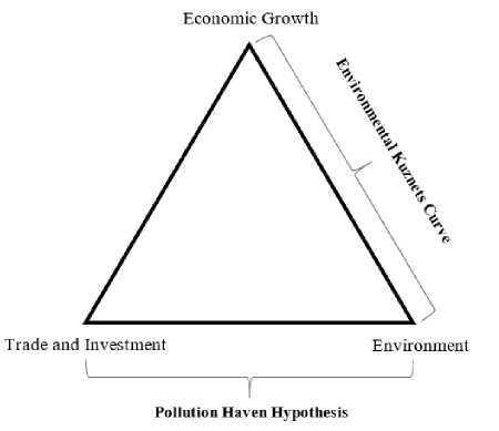
Figure 1. Trade-Environment Triangle

Source: Murthy & Gambhir (2017)

Murthy & Gambhir (2017) explain the relationship between environmental degradation, economic growth, and trade and investment into a framework called the trade-environment triangle. The framework explains that economic growth has two implications, namely on the environment and trade and investment (see Figure 1). On the one hand, this framework explains the relationship between economic growth and trade and investment. On the other hand, it also explains the relationship between the environment and economic growth. The use of these two relationships can explain the relationship between the environment

and trade and investment.

Several studies have analyzed the relationship between environmental degradation and various socioeconomic indicators. However, most studies only consider CO2 emissions as an indicator of environmental degradation and ignore other sources of environmental degradation. In fact, CO2 emissions are only part of environmental degradation. Therefore, CO2 emissions alone are not enough to be used as indicators in measuring environmental degradation (Nathaniel & Khan, 2020).

Researchers have recently begun to use the ecological footprint as a more comprehensive indicator in measuring environmental degradation caused by human activities (Destek & Sarkodie, 2019). Ecological footprint is a concept introduced by Wackernagel & Rees (1996) to calculate supply and demand from nature. On the demand side, the ecological footprint measures the amount of human consumption that comes from natural resources, such as food from plants, livestock and fish, wood and other forest products, land used for infrastructure development and waste generated from consumption activities. Meanwhile, on the

supply side, biocapacity calculates the amount of available natural resources that can be utilized by humans for consumption activities and also to absorb waste generated from consumption activities.

As a result of the process of industrialization and globalization that has continued to date, the world's economic growth has experienced rapid development. However, on the other hand, the burden on the environment is also increasing. According to the World Wildlife Fund or WWF (2020), through technological developments and better land management, global biocapacity has increased by about 28% in the last 60 years. However, the ecological footprint experienced a much faster increase with 173% or six times faster in the same period.

Indonesia is an interesting country to study for several reasons. First, Indonesia is the largest archipelagic country in the world and has the second longest coastline in the world (Coordinating Ministry of Maritime Affairs and Investment, 2018). Second, Indonesia is also the fourth most populated country in the world where

based on the results of the 2020 Population Census, 56.1% of the total population resides on the island of Java. Third, according to Kulp & Strauss (2019), Indonesia is one of the eight countries most affected by sea level rise due to climate change. As a result, sea level on the Indonesian coast will increase five to ten times by 2050. With these characteristics, Indonesia is one of the countries most vulnerable to the impacts of climate change.

On the economic side, in 2019, a real GDP of US$1.2 trillion made Indonesia the largest economy in Southeast Asia. However, despite Indonesia's rapid economic growth, on the other hand, Indonesia's ecological footprint has also experienced an increase that has exceeded its biocapacity since 2000. Therefore, the relationship between environmental degradation, economic growth and trade and investment in Indonesia is important to analyze.

In Indonesia itself, there are still few related studies that use the ecological footprint as an indicator of environmental degradation. Nathaniel (2020) analyzes the

relationship between the ecological footprint, economic growth, trade, energy consumption, and urbanization in Indonesia from 1971 to 2014. They found that economic growth, trade, energy consumption, and urbanization increase the ecological footprint in Indonesia.

Thus, there is a research gap that can be filled in this study, namely the analysis of the relationship between the ecological footprint as an indicator of environmental degradation with economic growth and trade and investment in Indonesia in a framework called the trade-environment triangle. Previous studies have also not analyzed the theory of EKC and PHH in Indonesia in a single analytical framework.

RESEARCH METHOD

Data

This study uses secondary time series data consisting of per capita ecological footprint, CO2 emissions per capita, per capita income as a proxy for economic growth, trade to GDP ratio, FDI to GDP ratio, PMTB ratio or investment to GDP, energy consumption per capita, the ratio of the urban population to the total population as a proxy for the level of

urbanization, and the human capital index.

The data were obtained from several

sources, namely the Footprint Network,

BP, World Bank Indicators (WDI), and the Penn World 10.0 Table developed by Feenstra et al. (2015) (see Table 1).

Table 1. Definition of Variables and Sources of Data

Variables	Symbol	Unit	Source
Ecological Footprint	EF	Global hectares per capita	Footprint Network
CO2 Emissions	C02	Metric tons per capita	BP
Gross Domestic Product	Y	Constant 2010 US$ per	WDI
(GDP)		capita
Trade	TR	(% from GDP)	WDI
Foreign Direct Investment	FDI	(%from GDP)	WDI
Gross Fixed Capital Formation (PMTB) or Investment	INV	(%from GDP)	WDI
Energy Consumption		Metric tons of oil	BP
	EN	equivalent
Urbanization Human Capital	URB	(% of total population)	WDI Penn World
	HC		Table10.0

studies, this study uses two indicators of environmental degradation, namely the ecological footprint and CO2 emissions so that there are four models which are

Model Spesification

This study follows the previous research model by Saboori et al. (2012) and Nathaniel (2020). In contrast to previous

estimated

as

follows:

Model 1:

EF_t = f(Y_t,Y_t∖TR_t,FDI_t,EN_t,URB_t,HC_t)

Model 2:

EF_t = f(Y_t,Y_t²,,TR_t,INV_t,EN_t,URB_t,HC_t)

Model 3:

C02_t = f(Y_t,Y_t²,TR_t,FDI_t,EN_t,URB_t,HC_t)

Model 4:

C02t = f(Yt,Yt²,TRt,INVt,ENt,URBt,HCt)

Furthermore, Chang et al. (2001) stated that the model converted into logarithmic form can reduce the stationarity problem

(1)

(2)

(3)

(4)

so that the equation model is obtained in logarithmic form. The equation is written as follows for simplification purposes:

Model 1:

InED¹_t = a_0i + a_{1 i}lnY_t + a_2ilnY_t² + a_3ilnTR_t + a₄ tlnFDI_t + a_silnEN_t + a_{6 i}lnURB_t + a_7ilnH C_t +

εtt                                                                                                                                            (5)

Model 2:

lnEDⁱ_t = β_0j + β_1jlnY_t + β₂jlnY_t² + β_3jlnTR_t + β_4jlnINV_t + β_sjlnEN_t + β_6jlnURB_t +

β7jlnHCt + εjt

Stationarity Test

There are various unit root tests that can be performed to test for stationary data, including Augmented Dickey-Fuller (ADF), Phillips-Peron (PP), and Kwiatkowski       Phillips-Schmidt-Shin

(KPSS). However, these three standard unit root tests do not have information related to structural breaks contained in the data so that the stationarity test results can be biased (Bahmani-Oskooee & Nasir, 2004). Therefore, in addition to using the three unit root tests, the Zivot-Andrews unit root test will also be used which includes one structural break.

Cointegration Test

The Autoregressive Distributed Lag (ARDL) method has several advantages over other cointegration test methods. First, this method can be used regardless of the stationarity test results for variables

(6) located at I(0), I(1) or a combination of both but not for variables that are stationary at I(2) (Pesaran & Shin, 1997). Second, an error correction model (ECM) can be generated from the ARDL model so that short-term information is obtained without losing long-term information. Third, this method can be used for research with a small sample (Pesaran & Shin, 1997). Fourth, there is no endogeneity problem because ARDL can eliminate serial correlation problems (Pesaran & Smith, 1998). Finally, estimation can still be done using the ARDL method even though the independent variable is endogenous (Pesaran et al., 2001; Pesaran & Shin, 1997).

Thus, the ARDL approach model from equations (5) and (6) is as follows:

MnEDⁱ_t = ^a₀i + ∑^p_k=₁ ^aM_kMnE I)-_c + ∑k=₀ ^a_2ikMnY- + ∑k=₀Onk (MnY_t-_k)² +

∑_k=o^a4t∣^Ml^nTRt-_k + ∑—^a5_!kMn^F∣)I— + ∑k=o^a6ik^∆lnENt-k + ∑kk=_oa_7lkMⁿURB_t-k +

∑‰₀a_8ikMnHC- + O_uInED- + θ_2ilnY- + O^lnY—)² + O_4lInTR- + O_5iInFDI- +

θ6_ilnEN- + O7ilnURBt-1 + O₈ilnHC- + ε_u                                                 (7)

MnEDt = β_0j + ∑hβij_lMnED- + ∑*=₀β₂μMnY- + ∑=₀β3j_i (MnY—)² +

∑=₀β₄j_lMnTR- + ∑=₀β_5jlMnINV- + Z=^j_lMnEN- + ∑=₀β_7μMnURB- +

∑‰ PsjMlnHC- + μijlnED- + μ₂jlnY- + μ3j(lnY-)² + μ₄jlnTR- + μ₅jlnINV- +

μ₆jlnEN- + μ7jlnURB- + μ_βjlnHC- + Ejt where p, q, r, s, t, u, v, and w are the optimal lags for each variable. In equations (7) and (8) have also included short-term and long-term estimates where the first difference variables (α and β} explain short-term estimates while O and μ explain long-term estimates.

Cointegration test is then carried out using F-statistics in which the hypotheses in this test are as follow:

Model 1:

H₀-.Oι =O2=O3 = O₄ = O₅ = O6 = O7 = O₈ = O

H₁: at least one O_i ≠ 0

Model 2:

^ho^i =μ2=μ3=μ4=μ5=μ6=μ7=μs = ⁰

H₁: at least one μ_i ≠ 0

by testing the null hypothesis, there is no cointegration against the alternative hypothesis there is cointegration. If the F-statistic value is lower than the critical value I(0) then the null hypothesis cannot

MnEDt = a₀i + ∑k=ι a_UkMnEF— + ∑k=₀ a2ikMnY-

(8)

be rejected, meaning that there is no cointegration between variables. However, if the F-statistic value is greater than the critical value I(1) then the null hypothesis is rejected, which means there is cointegration between variables.

After the cointegration test is performed and the long-term coefficient is obtained, then the error correction model (ECM) can be estimated to obtain the short-term coefficient. The ECM model of equations (5) and (6) is as follows:

+ ∑^rk=₀a3ik(ΛlnYt-i)²+                         (9)

∑k=o a4_lkΔlnTR_t-_k + ∑^t_k=₀ a_slkΔlnFDI_t-_k + ∑‰₀ ∑^=o a_8ik∆lnHCt-k + λECTt-ι + ⅜

∆lnEDt = βo_j + ∑^p_l=₁ βι_jl∆lnEF_t-_l + ∑=JF,_l∆lnιY-_l

∑f=oβ_4jl∆lnTR_t-_l + ∑^t_l=oβ_sjl∆lnINV_t._l + ∑Y=0β_6jl∆lnEN ∑‰β_8jl∆lnHC_t-_l + σECTt-ι + ε_jt

where λ and σ are the speed of adjustment coefficients indicating the speed of the variable returning to long-run equilibrium where the value of this coefficient must be statistically significant with a negative sign.

Diagnostic and Stability Tests

This study conducted several diagnostic tests, namely normality test, serial correlation test with Breusch-Godfrey, and heteroscedasticity test with Breusch-Pagan. Pesaran et al. (2001) also suggested a stability test with cumulative sum of recursive residuals (CUSUM) and cumulative sum of square of recursive residuals (CUSUMSQ).

a_6lk∆lnEN

t-k + ∑^vk=0a_7lk∆lnURBt-k +

'∑" β ■ (∆lnYt-l)² +

t-l + ∑r=0β_7jl∆lnURBt-l +

(10)

RESULTS AND DISCUSSION

Stationarity Test

Based on the results of the unit root test using four approaches, namely, ADF, PP, KPSS, and Zivot-Andrews, various results were obtained. The results of the stationarity test using the ADF, PP, and KPSS approaches are shown in Table 2 and the results of the stationarity test using Zivot-Andrews are in Table 3. It can be concluded that all variables are stationary at I(0) or I(1) using KPSS and Zivot-Andrews.

Table 2. Stationarity Test Results with ADF, PPS, and KPPS

Variables                  Intercept                        Intercept & Trend

	Level	1st Difference	Level	1st Difference
Augmented Dickey Fuller (ADF)
InEF	0,698	-7.016***	-2.969	-5.568***
InCO2	-2.862*	-5.930***	-0.610	-4.186**
InY	-0.666	-5.077***	-2.613	-5.036***
InY2	-0.279	-5.098***	-2.577	-5.040***
InTR	-3.308**	-8.790***	-2.895	-4.317***
InFDI	-2.698*	-3.964***	-3.422*	-3.912**
InINV	-2.001	-5.621***	-2.716	-5.574***
InEN	-2.616*	-6.266***	-0.393	-7.822***
InURB	-4.446***	-0.772	-0.180	-3.606**
InHC	-2.170	-0.535	0.030	-1.806
Phillips and Peron (PP)
InEF	0.787	-7.020***	-2.926	-7.414***
InCO2	-2.895*	-6.001***	-0.598	-7.193***
InY	-0.762	-5.045***	-2.258	-5.003***
InY2	-0.224	-5.067***	-2.192	-5.008***
InTR	-3.222**	-8.843***	-2.699	-10.080***
InFDI	-2.840*	-7.499***	-2.729	-7.459***
InINV	-2.497	-5.607***	-2.607	-5.561***
InEN	-2.616*	-6.357***	-0.394	-7.901***
InURB	-2.604*	-0.976***	1.462	-3.502*
InHC	-2.281	-0.567	2.392	-1.821
Kwiatkowski-Phillips-Schmidt-Shin (KPSS)
InEF	0.851	0,323***	0,152***	0,069***
InCO2	0.890	0,542***	0,212***	0,048***
InY	0.902	0,097***	0,115***	0,092***
InY2	0.903	0,090***	0,086***	0,090***
InTR	0.334***	0,287***	0,209***	0,074***
InFDI	0.112***	0,052***	0,111***	0,031***
InINV	0.530***	0,177***	0,106***	0,111***
InEN	0.875	0,458***	0,221***	0,052***
InURB	0.898	0,554***	0,210***	0,211***
InHC	0.870	0,529***	0,210***	0,183***

* p < 0.1, ** p < 0.05, *** p < 0.01

Table 3. Stationarity Test Results with Zivot-Andrews

Variables	Intercept                        Intercept & Trend Level         1st Difference         Level         1st Difference
InEF	-3.419                -8.032***           -3.381                -7.943***

	(2007)	(1997)	(2005)	(1997)
ItiCO2	-1.574	-4.601**	-2.314	-4.703
InY	(2004) -9.290***	(1989) -5.727***	(2004) -8.421***	(1989) -6.324***
InY2	(1998) -7.903***	(1997) -5.780***	(1998) -8.133***	(1998) -6.397***
InTR	(1998) -4.331	(1997) -9.476***	(1998) -6.252***	(1998) -9.760***
InFDI	(2009) -3.750	(1987) -8.100***	(1998) -4.093	(1987) -8.250***
InINV	(2004) -4.516	(2001) -6.513***	(1998) -5.064*	(2001) -6.558***
InEN	(1998) -2.916	(2004) -5.257**	(1998) -3.837	(2004) -4.443
InURB	(1989) -0.923	(1980) -7.696***	(2001) -3.907	(1989) -7.274***
InHC	(1988) -1.786	(2001) -4.631*	(1996) -2.745	(2001) -4.822*
	(2010)	(1981)	(2004)	(1981)

* p < 0.1, ** p < 0.05, *** p < 0.01

Cointegration Test

The next step, before the cointegration test is carried out using ARDL, is to determine the optimal lag for each estimated model. Optimal lag selection is done through unrestricted vector auto regression (VAR) with a maximum lag set of 2. Akaike Information Criteria (AIC) was chosen to determine the optimal lag for each model. Based on AIC, the optimal lag for all models is 2.

Based on the results of the cointegration test, the F-statistic value for Model 1 is 4.39, Model 2 is 6.35, Model 3 is 21.53, and Model 4 is 30.95 higher than the upper limit critical value at a significance level of 1% (4.26), so that the null hypothesis is rejected, which means that there is a cointegration or long-term relationship between the variables estimated for each model (see Table 4).

Table 4. Cointegration Test Results

ARDL models

lnEF, lnY, lnY², lnTR, lnFDI, lnEN, lnURB, lnHC (1, 1, 1, 1, 0, 1, 2, 0)

F-stat        Critical value bounds

Significance I(0)    I(1)

4.3992***          10%    2.03   3.13

lnEF, lnY, lnY2, lnTR, lnINV, lnEN, lnURB, lnHC (1, 2, 2, 1, 0, 2, 2, 0)	6.3592***	5%	2.32	3.50
lnCO2, lnY, lnY2, lnTR, lnFDI, lnEN, lnURB, lnHC (2, 1, 0, 0, 1, 2, 0, 1)	21.5384***	2.5%	2.60	3.84
lnCO2, lnY, lnY2, lnTR, lnINV, lnEN, lnURB, lnHC (2, 0, 0, 0, 1, 2, 0, 0)	30.9524***	1%	2.96	4.26

*** Significant at 1%

Long-Term and Short-Term Estimates

After performing the cointegration test, the next step is to interpret the long-term and short-term estimation results based on the ARDL model. The results of long-term and short-term estimates can be seen in Tables 5 and 6.

The estimation results show that the relationship between environmental degradation, using both the ecological footprint and CO2 emissions as indicators of environmental degradation, and economic growth in Indonesia, is a U-shaped relationship in the long term. This result means that in the early stages of economic growth, environmental degradation decreases as income increases and after a certain point it increases as

income increases. These results do not support the existence of EKC in Indonesia. This finding is in line with previous studies by Saboori et al. (2012) and Azwar (2019) in Indonesia.

Azwar (2019) explained that the reason the EKC theory does not apply in Indonesia is because the Indonesian economy is still dominated by resource-intensive sectors compared to services-intensive sectors. The resource-intensive sector, such as the agriculture, forestry, and fishery as well as the industrial sector including the manufacturing, mining, and construction, electricity, water and gas sectors contributed to 51.67% of Indonesia's total GDP in 2019. Services contributed to 44.23% of Indonesia's total GDP in 2019.

Table 5. Long-term Estimation Results

Dependent Variables : Ecological Footprint					Dependent Variables: CO2 Emissions
Model 1			Model 2		Model 3		Model 4
	Coefficient	t-stat	Coefficient	t-stat	Coefficient	t-stat	Coefficient	t-stat
InY	-6.370**	-2.344	-7.913***	-4.167	-7.643***	-5.761	-5.204***	-4.623
		(0.026)		(0.000)		(0.000)		(0.000)
InY2	0.433**	2.520	0.563***	4.593	0.500***	5.706	0.366***	4.993

		(0.017)		(0.000)		(0.000)		(0.000)
InTR	0.084	1.598	0.056*	1.727	0.210***	4.580	0.182***	4.030
		(0.120)		(0.095)		(0.000)		(0.000)
InFDI	-0.015	-1.236			0.011	1.118
		(0.226)				(0.272)
InINV			-0.289***	-4.516			-0.170***	-3.114
				(0.000)				(0.004)
InEN	0.111	0.578	0.259**	2.075	1.105***	11.872	1.040***	11.366
		(0.568)		(0.047)		(0.000)		(0.000)
InURB	-0.180	-0.377	-1.320***	-2.962	-0.105	-0.280	-1.006**	-2.541
		(0.709)		(0.006)		(0.782)		(0.016)
InHC	0.595	0.984	1.662***	3.420	0.381	0.8080	1.338***	2.928
		(0.333)		(0.002)		(0.426)		(0.006)

* p < 0.1, ** p < 0.05, *** p < 0.01, values in brackets are p-value

Furthermore, the estimation results show that trade significantly increases the ecological footprint and CO2 emissions in Indonesia in the long term. This result reveals that trade liberalization actually increases environmental degradation in Indonesia. In 2019, total trade contributed to 37.3% of the total GDP of which 19% came from imports and 18% came from exports. Furthermore, imports are dominated by industrial products, such as electrical equipment, measuring

instruments, and optics (14.2%), base metal products (13%), and oil and gas (12.7%). Meanwhile, exports were dominated by coal (13.9%), palm oil (9.4%), and oil and gas (7%). These digits show that most of Indonesia's trade products come from resource-intensive sectors. Thus, the scale effect of trading still dominates over the compositional effect and the technical effect. These findings are in line with Saboori et al. (2012) in Indonesia and Lanouar (2017) in Qatar.

Table 6. Short-term Estimation Results

Dependent Variable: Ecological Footprint					Dependent Variable: CO2 Emissions
	Model 1		Model 2		Model 3		Model
	Coefficient	t-stat	Coefficient	t-stat	Coefficient	t-stat	Coefficient	t-stat
D(InY)	1.279	0.313	0.971	0.239	-1.897	-0.701	-0.928	-0.403
		(0.756)		(0.813)		(0.489)		(0.690)
D(lnY2)	-0.052	-0.194	-0.016	-0.059	0.132	0.740	0.075	0.496
		(0.848)		(0.953)		(0.465)		(0.624)
D(InTR)	0.035	0.982	0.076**	2.286	0.057	1.597	0.050	1.479
		(0.334)		(0.031)		(0.121)		(0.149)

D(InFDI)	0.002   0.336                               0.004   0.613 (0.739)                                           (0.544)
D(InINV)	-0.118*   -1.708                                -0.055   -1.011 (0.100)                                           (0.320)
D(InEN)	-0.230**   -2.538        -0.145   -1.662      0.971***   8.279      0.866***  10.114 (0.017)                  (0.109)                  (0.000)                  (0.000)
D(InURB)	3.927**   2.054       3.944*   2.036        -1.383   -1.307       -1.637   -1.638 (0.049)                  (0.052)                  (0.202)                  (0.112)
D(InHC)	0.462   0.611        1.347   1.490        1.982   1.419        1.064   1.299 (0.546)                  (0.148)                  (0.167)                  (0.204)
C	-0.004   -0.247        0.001   0.046        0.023   1.263        0.020   1.141 (0.807)                  (0.964)                  (0.217)                  (0.263)
ECT(-1)	-0.491***   -2.446     -0.728***   -2.718     -0.587***   -3.423     -0.667***   -3.733 (0.021)                  (0.012)                  (0.002)                  (0.001)
R2 Adjusted R2	0.611                 0.711                 0.871                 0.876 0.409                 0.512                 0.805                 0.825

* p < 0.1, ** p < 0.05, *** p < 0.01, values in brackets are p-values

The estimation results also show that the relationship between environmental degradation, both using the ecological footprint and CO2 emissions as indicators of environmental degradation, and FDI in Indonesia has not shown statistically significant results. Thus, it cannot be concluded that the existence of PHH in Indonesia has not been shown. Dean (2001) and Jaffe et al. (2013) stated that environmental regulation is not the only factor that is considered by investors in determining the location of investment. There are other factors that are also taken into consideration, such as cheap and skilled labor and the quality of infrastructure. These findings are in line with Shofwan & Fong (2014) in Indonesia.

This aspect is different from the overall investment where the estimation results show that the investment significantly reduces the ecological footprint and CO2 emissions in Indonesia in the long term. These results indicate that the existing investments have been allocated to finance environmentally friendly projects so as to reduce environmental degradation. These findings are in line with Zubair et al. (2020) in Nigeria.

Economic growth is inseparable from other factors that also affect the quality of the environment. The estimation results show that energy consumption significantly increases the ecological footprint and CO2 emissions in Indonesia

in the long and short terms. This condition is because Indonesia's energy consumption is still dominated by non-renewable energy consumption which reached 93.91% in 2019. These findings are in line with Saboori et al. (2012) and Nathaniel (2020) in Indonesia.

Furthermore, it is undeniable that high economic growth can encourage the flow of urbanization which in turn can also affect the quality of the environment. The estimation results show that urbanization significantly reduces the ecological footprint and CO2 emissions in Indonesia in the long term. These findings are in contrast to Nathaniel's previous research (2020) which found that urbanization has a positive relationship with the ecological footprint in Indonesia from 1971 to 2014. However, this finding is supported by Arouri et al. (2014), Dogan et al. (2019), and Martínez-Zarzoso & Maruotti (2011). Martinez also found that the high levels of urbanization in developing countries are related to negative impact on environmental degradation. This condition is because urbanization can increase economies of scale and thus, the goal of

improving environmental quality can be achieved.

Diagnostic and Stability Tests

The diagnostic test for each estimated model last is the last step. There are three diagnostic tests carried out, namely normality test, serial correlation test, and heteroscedasticity test. The results of the diagnostic test can be seen in Table 7. It can be concluded that the error terms in all models are normally distributed, there are no serial correlation and heteroscedasticity problems. Finally, the estimation results show that human capital significantly increases the ecological footprint and CO2 emissions in Indonesia in the long term. This finding is in line with Malik et al. (2020) in Pakistan. This condition is because high human capital does not necessarily change human behavior in consuming energy. There are other factors, such as energy prices that can affect human behavior (Ohler & Billger, 2014).

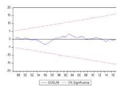
In addition, stability tests were also carried out on each estimated model using the CUSUM and CUSUM-SQ tests. The stability test results can be seen in Figure 2. The stability test results show that for all

models, the CUSUM and CUSUM-SQ lines models are stable at the 5% level. are within the critical limit so that all

Table 7. Diagnostic and Stability Tests

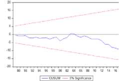
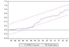
Figure 2. Plot CUSUM and CUSUM-SQ

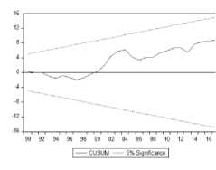
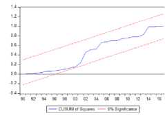
Plot CUSUM and CUSUM-SQ Model 1

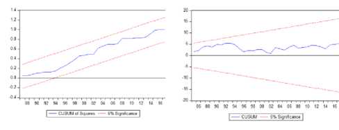
Plot CUSUM and CUSUM-SQ Model 2

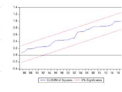
Plot CUSUM and CUSUM-SQ Model 3

Plot CUSUM and CUSUM-SQ Model 4

	Model 1	Model 2	Model 3	Model 4
Normality Test	1.333	0.196	0.179	0.703
	(0.514)	(0.907)	(0.914)	(0.704)
Serial Correlation Test	1.048	1.110	0.574	1.628
	(0.363)	(0.345)	(0.567)	(0.213)
Heteroscedasticity test	0.787	0.817	0.455	0.763
	(0.675)	(0.663)	(0.940)	(0.683)
CUSUM	Stable	Stable	Stable	Stable
CUSUM-SQ	Stable	Stable	Stable	Stable

values in brackets are p-values

also examines the existence of the EKC and

PHH theories in Indonesia in a framework

CONCLUSION

This study aims to analyze the relationship between environmental degradation and economic growth and trade and investment in Indonesia from 1970 to 2017. In contrast to previous studies, this study

called the trade-environment triangle. The relationship between these variables was estimated using the ARDL method.

This study uses aggregated data at the national level due to the limitations of data for the provincial level so that in the future

similar research can be carried out at the provincial level. Also,

using data on the ratio of incoming FDI to GDP, this study has not been able to explain the existence of PHH in Indonesia. Therefore, further research can try to explain the existence of PHH in Indonesia using other data, such as incoming FDI by sector.

However, there are some important results from the research that can be taken into account. Based on the estimation results, the relationship between environmental degradation and economic growth is a U-shaped relationship, meaning that there is no EKC in Indonesia. The relationship between environmental degradation and FDI in Indonesia is also not statistically significant so that the existence of PHH in Indonesia cannot be explained. The estimation results also show that trade, energy consumption, and human capital significantly increase environmental degradation in Indonesia in the long term. In contrast, investment and urbanization significantly reduce environmental degradation in Indonesia in the long run.

From the results of the analysis, several policy implications can be explained. First, there is no EKC presence in Indonesia, meaning the government can consider encouraging economic growth so that it does not only depend on resourceintensive sectors. The service sector and clean industry can also be encouraged to achieve sustainable economic growth. Second, trade liberalization in Indonesia increases environmental degradation so that the government can consider making trade strategies that can increase environmental     protection.     Third,

investment in Indonesia reduces environmental degradation so that the government can create a better investment climate in order to attract both local and foreign investors so that existing investments can be allocated to the development of more environmentally friendly projects.

REFERENCES

Arouri, M., Shahbaz, M., Onchang, R., Islam, F.,  & Teulon, F. (2014).

Environmental Kuznets Curve in Thailand: Cointegration and Causality Analysis. IPAG Working Paper.

Azwar. (2019). Economic Growth and Co2

Emissions in Indonesia : Investigating

the Environmental Kuznets Curve Hypothesis Existence. Jurnal BPPK: Badan Pendidikan Dan Pelatihan Keuangan,        12(1),        42–52.

https://doi.org/10.48108/jurnalbppk. v12i1.369

Bahmani-Oskooee, M., & Nasir, A. B. M. (2004). ARDL approach to test the productivity bias hypothesis. Review of Development  Economics,  8(3),  483–

488.https://doi.org/10.1111/j.1467-9361.2004.00247.x

Chang, T., Fang, W., & Wen, L. (2001). Energy consumption, employment, output, and temporal causality: evidence from Taiwan based on cointegration  and  error-correction

modelling    techniques.    Applied

Economics,      33(8),      1045–1056.

https://doi.org/10.1080/00036840122 484

Copeland, B. R., & Taylor, M. S. (1994). North-South Trade and the Environment. The Quarterly Journal of Economics, 109(3), 755–787. Retrieved from

http://www.jstor.org/stable/2118421

Dean, J. M. (2001). International Trade and Environment. UK: Ashgate Publisher.

Destek, M. A., & Sarkodie, S. A. (2019). Investigation of environmental Kuznets curve for ecological footprint: The role of energy and financial development. Science of the Total Environment,     650,     2483–2489.

https://doi.org/10.1016/j.scitotenv.20 18.10.017

Dogan, E., Taspinar, N., & Gokmenoglu, K. K. (2019). Determinants of ecological footprint in MINT countries. Energy

and    Environment,    30(6),    1–22.

https://doi.org/10.1177/0958305X198 34279

Feenstra, C., R., Inklaar, R., & Timmer, M. P. (2015). No TitleThe Next Generation of the Penn World Table. Americam Economic Review, 105(10),

3150–3182.      Retrieved      from

www.ggdc.net/pwt

Grossman, G. M., & Krueger, A. B. (1991). Environmental Impacts of a North American Free Trade Agreement. NBER Working Papers, (3914).

IPCC. (2007). Climate Change 2007: Synthesis Report. Contribution of Working Groups I, II and III to the Fourth Assessment     Report     of     the

Intergovernmental Panel on Climate Change [Core Writing Team, Pachauri, R.K and Reisinger, A.    (eds.)].

https://doi.org/10.1038/446727a

IPCC. (2014). Climate Change 2014 Synthesis Report Summary Chapter for Policymakers.

IPCC. (2018). Summary for Policymakers. In: Global Warming of 1.5°C. An IPCC Special Report on the impacts of global warming of 1.5°C above pre-industrial levels and related global greenhouse gas emission pathways, in the context of strengthening the global response to.

Jaffe, A. B., Peterson, S. R., Portney, P. R., & Stavins, R. N. (2013). Environmental Regulation and the Competitiveness of U.S. Manufacturing: What Does the Evidence Tell Us? American Economic Association, 33(1), 132–163.

Kemenko Bidang Kemaritiman dan Investasi. (2018). Menko  Maritim

Luncurkan Data Rujukan Wilayah

Kelautan Indonesia. Retrieved from https://maritim.go.id/menko-maritim-luncurkan-data-rujukan-wilayah-kelautan-indonesia/

Kulp, S. A., & Strauss, B. H. (2019). New elevation data triple estimates of global vulnerability to sea-level rise and coastal flooding. Nature Communication.

https://doi.org/10.1038/s41467-019-12808-z

Lanouar, C. (2017). The impact of energy consumption     and     economic

development on Ecological Footprint and CO2 emissions: Evidence from a Markov Switching Equilibrium Correction Model. Energy Economics. https://doi.org/10.1016/j.eneco.2017. 05.009

Malik, M. Y., Latif, K., Khan, Z., Butt, H. D., Hussain, M., & Nadeem, M. A. (2020). Symmetric and asymmetric impact of oil price, FDI and economic growth on carbon emission in Pakistan: Evidence from ARDL and non-linear ARDL approach. Science of the Total Environment,  726(April).

https://doi.org/10.1016/j.scitotenv.20 20.138421

Martínez-Zarzoso, I.,  & Maruotti, A.

(2011). The impact of urbanization on CO2 emissions:   Evidence from

developing countries. Ecological Economics,      70(7),      1344–1353.

https://doi.org/10.1016/j.ecolecon.20 11.02.009

Murthy, K. V. B., & Gambhir, S. (2017). International trade and foreign direct investment: empirical testing of the trade–environment          triangle.

Transnational Corporations Review, 9(2), 122–134.

https://doi.org/10.1080/19186444.20 17.1326718

Nathaniel, S., & Khan, S. A. R. (2020). The nexus     between     urbanization,

renewable   energy,   trade, and

ecological   footprint   in ASEAN

countries. Journal of Cleaner Production, 272.

https://doi.org/10.1016/j.jclepro.2020 .122709

Nathaniel, S. P. (2020). Ecological footprint, energy use, trade, and urbanization linkage in Indonesia. Geo Journal,                                  7.

https://doi.org/10.1007/s10708-020-10175-7

Ohler, A. M., & Billger, S. M. (2014). Does environmental concern change the tragedy of the commons? Factors affecting energy saving behaviors and electricity usage. Ecological Economics, 107,                               1–12.

https://doi.org/10.1016/j.ecolecon.20 14.07.031

Pesaran, M. Hahem, Shin, Y., & Smith, R. J. (2001). Bounds Testing Approaches to the Analysisi of Level Relationships. Journal of Applied Econometrics, 16, 289– 326. https://doi.org/10.1002/jae.616

Pesaran, M. Hashem, & Shin, Y. (1997). An Autoregressive Distributed Lag Modelling Approach to Cointegration Analysis. Econometrics and Economic Theory in the 20th Century: The Ragnar Frisch      Centennial     Symposium.

https://doi.org/10.1017/ccol05216332 30.011

Pesaran, M Hashem, & Smith, R. P. (1998). Structural Analysis of Cointegration VARs. Journal of Economic Surveys, 12(5), 471–505.

Saboori, B., Sulaiman, J. Bin, & Mohd, S. (2012). An Empirical Analysis of the Environmental Kuznets Curve for CO2 Emissions in Indonesia: The Role of Energy Consumption and Foreign Trade. International Journal of Economics and Finance, 4(2), 243–251. https://doi.org/10.5539/ijef.v4n2p24 3

Shofwan, S., & Fong, M. (2014). Foreign Direct Investment and the Pollution Haven Hypothesis in Indonesia. Journal of Law and Governance, 6(2), 27– 35. https://doi.org/10.15209/jbsge.v6i2.2 02

Wackernagel, M., & Rees, W. (1996). Our Ecological Footprint: Reducing Human Impact on the Earth. New Society Publishers.

WWF. (2020). Living Planet Report 2020 -Bending the curve of biodiversity loss. Gland, Switzerland: WWF.

Zubair, A. O., Samad, A.-R.  A.,  &

Dankumo, A. M. (2020). Does gross domestic income, trade integration, FDI inflows, GDP, and capital reduces CO2 emissions? An empirical evidence from Nigeria. Current Research       in       Environmental

Sustainability,                           2.

https://doi.org/10.1016/j.crsust.2020. 100009

20