RETRIEVAL OF SURFACE CURRENT FROM HIMAWARI-8 SEA SURFACE TEMPERATURE DATA AND PARTICLE IMAGE VELOCIMETRY METHOD
on
Retrieval of Surface Current From Himawari- Sea Surface...,
[Kadek Setiya Wati, dkk]
RETRIEVAL OF SURFACE CURRENT FROM HIMAWARI-8
SEA SURFACE TEMPERATURE DATA AND PARTICLE IMAGE VELOCIMETRY METHOD
Kadek Setiya Wati1*), Takahiro Osawa2), I Wayan Gede Astawa Karang3)
-
1)Indonesian Agency for Meteorological Climatological and Geophysical (BMKG).
-
2)Center of Research and Application of Satellite Remote Sensing (YUCARS), Yamaguchi University, Ube-Shi Yamaguchi Japan.
-
3)Department of Marine Sciences, Faculty of Marine Science and Fisheries, Udayana University, Denpasar, Bali, Indonesia.
*Email: kadek.setiya@gmail.com
ABSTRACT
As human activity occurs at the surface, which is influenced by surface currents, understanding surface currents is crucial. Ocean currents are not solely caused by wind, but also of other factors, such as sea surface temperature. To obtain surface current data, BMKG used HF radar installed in several places, including Flores Sea. This location is significant because it has large ports and heavy crossing traffic. This study aims to analyse surface current data retrieve from Himawari-8 SST data by applied PIV algorithm. Using the PIV algorithm, a cross-correlation plane is generated by comparing two identically sized interrogation windows obtained from successive images. On 5 December 2022 in the Flores Sea, Himawari-8 SST data was employed to estimate sea surface currents every 10 minutes. Surface current motion varies widely from image to image. Western areas are dominated by westward currents, while central and eastern areas are dominated by eastward currents during daylight hours, and westward currents during the night. Synoptic wind affects surface current movement during those hours. Validation with observational data from the Labuan Bajo HF radar shows that the V component current estimation is better than the U component current estimation. This is particularly prevalent in the south and in areas close to the KAWA radar HF location. Keywords: Flores Sea; SST; Himawari-8; PIV; surface current
The surface currents are driven by wind, but other factors, such as sea surface temperature, also play a significant role. Various atmospheric heat fluxes, diffusion, and advection influence changes in ocean temperatures over time (Rio et al., 2016). Oceanic circulation has a substantial influence on sea surface temperatures in most of the equatorial Pacific. A study by Bonjean (2001), showed that surface zonal advection (from surface currents observation) is essential
in large-scale changes in SST distribution. Furthermore, a study conducted by Peng et al. (2022) using the Ocean General Circulation Model (OGCM) found that ocean current change is influenced by SST changes. The model estimates that a change in SST accelerates upper ocean currents in 77% of the global ocean, significantly more than a change in wind forcing.
It is essential to understand surface currents in order to solve environmental problems. Ocean currents can move debris thousands of kilometers from their source, making it a global environmental problem
(Wichmann et al., 2019). As marine debris is found throughout the ocean and carried by currents to multiple destinations, it is ubiquitous and transboundary (Purba et al., 2019). In addition to facilitating the transport of marine debris, ocean surface currents also play a role in distributing nutrients. Surface currents play a significant role in the transfer of nutrients, according to Dorofeyev and Sukhikh (2019).
Due to two types of issues, surface current processes are more difficult to resolve using in situ data. As a result of limited spatial and temporal resolutions, we cannot calculate surface currents precisely. Second, collecting in situ data requires time and money (Ghalenoei & Hasanlou, 2017).
Over the last few decades, various approaches and methodologies have been proposed to determine surface currents from surface tracers such as sea surface temperature (SST) or ocean color (OC) (González-Haro et al., 2020). The large-scale particle image velocimetry technique can be used to determine sea surface flow conditions in the oceanographic environment (Choi et al., 2021; Perkovic et al., 2009; Russmeier et al., 2017). There is a need for high-resolution temporal LSPIV observations to provide enough data for consistent in situ validation. The ADCP's consistent in-field observations revealed that both systems agree with accurate measurements of sea surface flow directions (Russmeier et al., 2017).
Real-time observations of surface currents are currently being conducted in Indonesia using HF radar. Despite this, this tool has been installed at four locations, including the Flores Sea. Due to the limitations and high cost of in-situ measurements, a strategy is required to resolve this issue. Himawari-8 geostationary satellite is one of the remote sensing devices capable of continuous observation and high spatial (2 km) and
temporal resolution (10 minutes). This satellite has been used to estimate ocean currents in a variety of ways. The purpose of this study is to retrieve high resolution of surface current from Himawari-8 and analyst the distribution of surface current in the Flores Sea based on Himawari-8 data. In this case, the PIV method is combined with Sea Surface Temperature (SST) data. It is expected that this approach could be used as an alternative method in BMKG operations. It provides high resolution surface current data. A number of applications can be made of these surface current data, including analyzing ship accidents, supporting ship information, and marine tourism.
The Flores Sea will serve as the location for the investigation; its coordinates range from 7.5 S to 9.0 S and 119 E to 123 E. It is bordered by the Bali Sea on the west and the Banda Sea on the east. These two seas form the boundary of the Flores Sea. Meanwhile, Sulawesi is located in the north of this region, while Flores is located in the south. The region surrounding this area is home to one of the most renowned tourist destinations in Indonesia, Komodo National Park.
In this study, the research date, 5 December 2022, was chosen based on consideration of the minimum cloud cover conditions around the research location during the 2022/2023 rainy season. This period as a representation of the Asian monsoon in Indonesia as well as to explore the potential of this method to be applied during the rainy season.
Specifically, SST data from Himawari-8 were used in this study. In this study, this data serves as an independent variable. Afterwards, two successive images are used with a 10-minute interval. In order to produce a
velocity vector chart, each image will be pre-processed and calculated based on a cross-correlation algorithm. The estimation results will proceed through a post processing process, namely filtering and smoothing to remove incorrect vectors. Utilizing HF radar data as a control variable, data processing results in a vector velocity chart that provides the dependent variable. After obtaining the final estimation results, a comparison is made between ocean current data provided by estimates and real-time observations by HF radars. Several statistical methods are used at this stage.
Furthermore, the daily distribution of estimated surface current data is also compared with synoptic wind conditions. Based on the results obtained, it is expected that this method will be applied to BMKG operations. There are many useful applications that can be made of surface current data, including the analysis of ship accidents, the support of ship information, and the provision of marine tourism equipment, which can be taken advantage of based on the data that have been produced. Figure 1 shows the concept of this research.
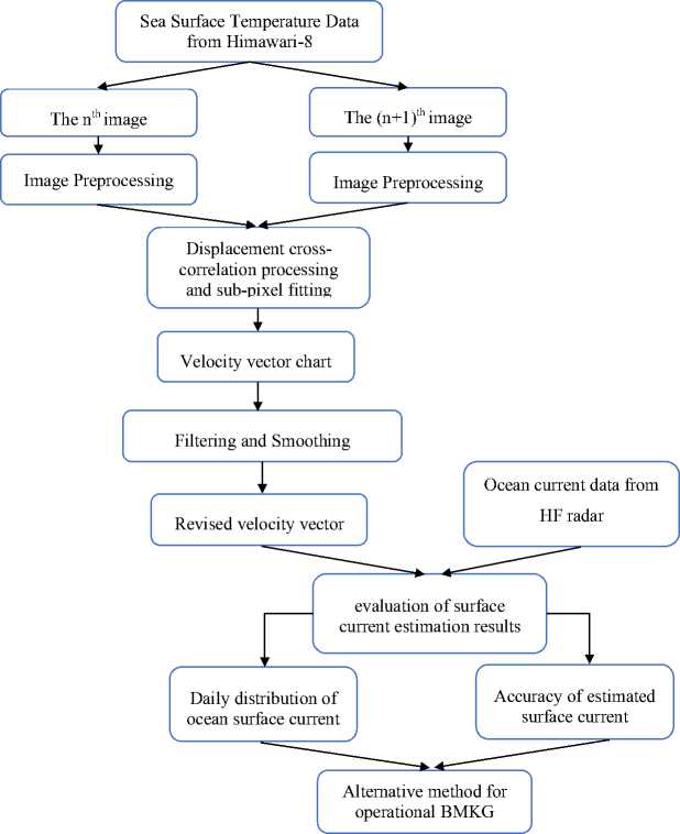
Figure 1. Research concept
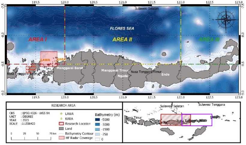
Figure 2.
Research Area (purple rectangle) is divided into 3 sub areas (area I, area II, area III). HF radar coverage (red square) as validation area.
The study utilized the following data:
-
1. The SST level 2 data from Himawari-8 with a time resolution of 10 minutes and a spatial resolution of 2 km. The data were produced by JAXA Himawari Monitor System and downloaded from the website
http://www.eorc.jaxa.jp/ptree/index. html.
-
2. Data observations of ocean surface currents from HF radar. Figure 2 shows the two-point location and coverage area of the Labuan Bajo HF radar. HF radar at Labuan Bajo uses 13 MHz frequency. Those data have a spatial resolution of 1 km and a temporal resolution of 20 minutes. HF radar data in the Flores Sea were obtained from the BMKG Marine Meteorological Centre.
-
3. Additionally, to support this analysis, an analysis map is used for the 10 m layer that represents wind
speed and direction based on the IFS 0.125 model from BMKG, and a surface current direction and speed based on the Wave Watch III model from BMKG OFS.
Two consecutive images are used in the PIV method to measure image pixels movement. There is a sizeable disk area of SST data, in netCDF format. In the first step, the site is segmented according to the research area. After cutting the data, the projection map is adjusted so that the Himawari SST data is projected using the WGS84 (World Geodetic System 1984) projection map. As a step, the SST unit converted from Kelvin to Celsius. SST distribution is displayed at intervals of 0.4°C. After that, the map is saved in image format to be used in the following process. This step is repeated for the whole study data.
Refers to Fujita et al. (1998), crosscorrelation is used to determine the interrogation area (IA) in the first image, as well as the interrogation area in the
search area (SA) in the second image. An Equation 2 shows the cross-correlation of a pair of particles to determine a candidate vector (Balamurugan & Jeeva, 2019):
R(S,t)= ∑ 7⅛ ∑ Jto1 fI,j (i, j)f; , 'j(i+s,j+t) (1)
Where
R is the recurrent cross-correlation
between sub-windows I, J in the first image of the image pair (F') and the next image of the image pair (F"),
i j is the pixel location within subwindows I, J, and
s, t is the 2-D cyclic lag for that crosscorrelation computing.
For discrete data, the Fourier transform is
efficiently implemented using the Fast Fourier transform, which reduces computation operations.
An interrogation window
subsamples two sequential digital images, where the correlation peak directly correlates with particle displacement. This formula calculates particle average velocity (Hsu et al., 2011):
—→
→ Δ ⃗⃗
v⃗=
∆t
Where:
ΔХ is the average spatial shift;
(2)
Δt is the time interval between two
sequential images.
This study uses a multipass scheme interrogation window: pass 1: 128 x 128, pass 2: 64 x 64, and pass 3: 32 x 32 with 50% overlap. Moreover, the crosscorrelation distribution is fitted with Gaussian fitting to improve measurement accuracy by subpixel peak detection (Fujita et al., 1998). The analysis process is carried out using PIVlab software. Moreover, PIVlab uses pixels per frame as its units, so a calibration is performed to compare the distance represented by one pixel to the actual distance. It is necessary to determine two reference points where the distance between images can be determined (in mm) and the time step between images can be determined (in
ms). Post-processing steps by using median filtering and data smoothing were applied to reduce errors.
The calculations conducted to get the value of ocean current speed using Equation 3 and Equation 4 (Supriyadi et al., 2021):
curr =√U2 + V2 (3)
θ= (4)
U
Where:
The curr is current sea speed (m/s) θ is the current sea direction (degree) u is the zonal current
v is the meridional current
To evaluate the accuracy of estimated surface current data, validate with HF radar data by using equations 5 and 6 below:
e =√1∑F (
crms=∑( mean
bias = ∑i=i estimated, i
Where
-
A2 estimated, i) (5)
true value (6)
-
destimated,i is the displacement estimated by PIV at observation i,
dtrue value is the true displacement,
dmean is the mean of estimated
displacement, and
n is the total number of observations.
Estimating surface current velocity using SST data and the PIV method was performed at 10-minute intervals on each selected research date. Estimation data is then displayed as a current rose to describe the average percentage of surface current movement in a day. This is done in each area of the Flores Sea. The current rose is a diagram showing the average proportion of the current setting toward each significant compass point in a specified marine area. The effect of tidal currents was not considered in this analysis due to their negligible effect on the open sea and processing of the data in the context of daily averages.
Since the study area is quite large and the surrounding seas have different influences, the study area between 7.5° – 8.5° South and 119° – 123° East is divided into three parts, including the western part (area 1) covering coordinates 7.5°–8.5° S and 119°–120° E; the central part (area 2) includes coordinates 7.5°–8.5° S and 120°–122° E; and the eastern part (area 3) includes coordinates 7.5°– 8.5° S and 122°–123° E (see Figure 2). The movement of surface currents in each area is then displayed as a current rose every 3 hours. The time classification for the analysis is as follows: 00-03 UTC and 0306 UTC represent the morning; 06-09 UTC and 09-12 UTC represent noon; 1215 UTC and 15-18 UTC represent nighttime; 18-21 UTC and 21-24 UTC represent early morning.
Figures 3 and Figure 4 show that ocean surface currents moved varied on 5 December 2022. The percentage of the total daily average flow of surface currents in this period is 28-35% heading west, 14-21% heading east and the rest is North-South currents.
The western part of the Flores Sea shows that surface currents move in highly variable directions, especially in the morning and afternoon. During this time, zonal and meridional flows can be observed. In the morning and afternoon, surface currents move in the zonal direction by 14-26% and 7-17% in the meridional direction. In the morning, 1925% of surface currents head West, and 14-15% head East. Meridional flow is dominated by southward movement (917%). This condition is still visible during the day, with an increase of 1% for flows to the West and 5% for flows to the East. Northward flow predominates at this time (10-17%). At night, the dominant surface current shift to the East at 12-15 UTC (2835%). At 15-18 UTC, the current reversed again towards the West. This condition lasted until early morning with a
percentage of 24-55%. In the early morning, meridional variations are minimal during this period.
On the other hand, the central part of the Flores Sea shows slightly different conditions. Ocean surface currents are generally dominant in the zonal direction but in the opposite direction, namely eastward. In the morning, ocean surface currents vary widely. Surface currents move in zonal and meridional directions, with respective percentages of 18-30% and 9-16%. The dominant surface current is towards the East at this time, and the meridional flow is dominated by the South. Conditions during the day appear similar to those in the morning. Ocean surface currents tend to move primarily to the East and also significantly meridionally. If surface currents drift south in the morning, conditions change to the north during the day. Similar to conditions in the western part of the Flores Sea, at night, there is a meridional decrease in flow and a zonal strengthening of the flow. At 12-15 UTC, the dominant current is heading East (30-35%), and starting at 15-18 UTC, the dominant current is moving West. This condition persists until the early morning hours with an incidence percentage of 40-70%.
In general, in the eastern part of the Flores Sea, ocean surface currents still predominantly move in a zonal direction. Conditions in the morning looked like conditions in the central Flores Sea. Ocean surface currents move in widely varying directions. Even though zonal currents dominate, especially to the East (20-30%), meridional currents are also significant. However, surface currents heading north and south are balanced. These conditions continued until 06-09 UTC. In the next 3 hours, at 09-12 UTC, the current movement seemed increasingly erratic because the currents seemed to be moving towards the West, North, and South with almost the same number of occurrences with a
difference in the percentage of events of less than 10%. Even though it tends to be random, ocean surface currents are more likely to be east (22%). At night, the meridional flow weakened, and the zonal flow strengthened again. The previously dominant ocean surface currents headed
east gradually reversed their direction and became primarily westward. The ocean surface currents that move towards the East decrease in number in the early morning hours, and the meridional currents do. Ocean surface currents leading to the West are dominant in this period, by 24-60%.
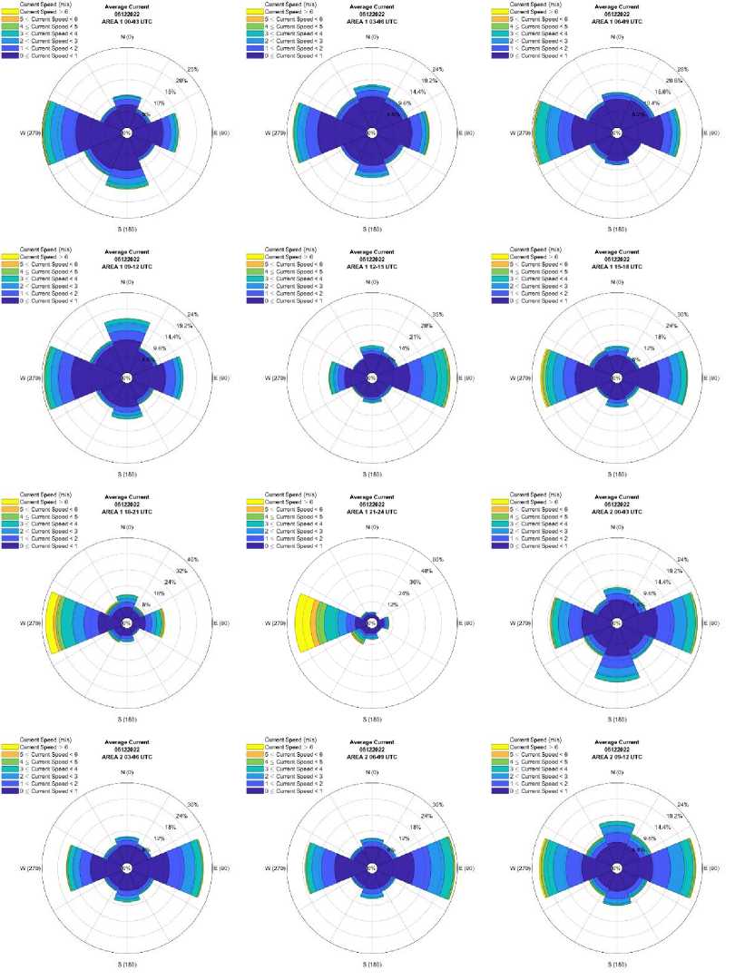
Figure 3.
Current Rose of estimated surface currents on 5 December 2022
in the Area 1 at 00-24 UTC and Area 2 at 00-12 UTC.
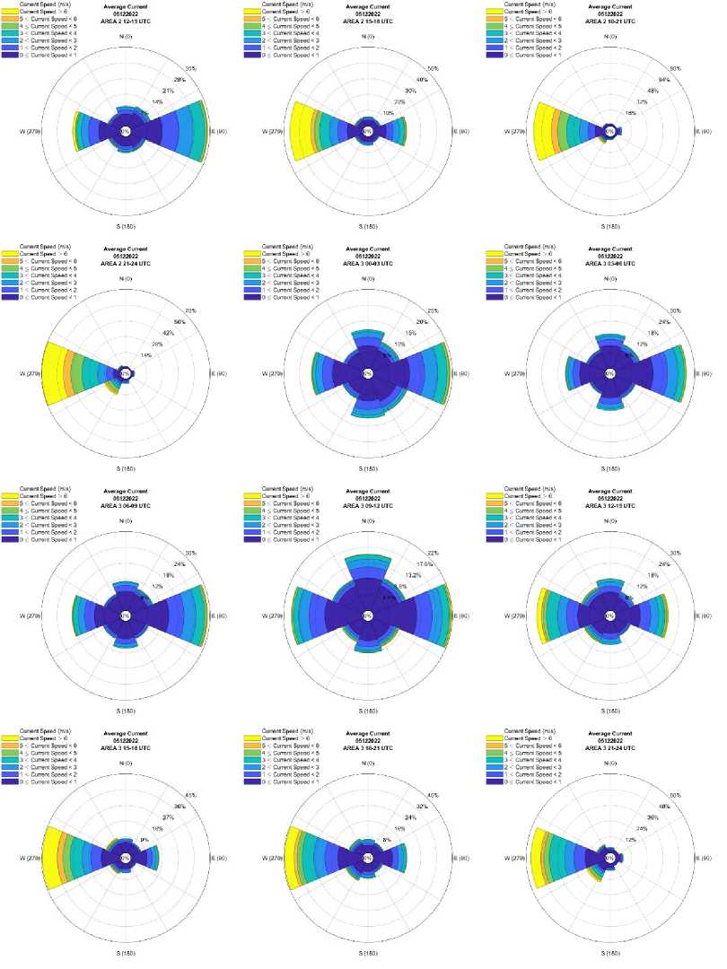
Figure 4.
Current Rose of estimated surface currents on 5 December 2022
in the Area 2 at 12-24 UTC and Area 3 at 00-24 UTC.
As a representation of the Asian Monsoon period, the movement of ocean surface currents on 5 December 2022 is dominated by zonal or east-west movement. A zonal component dominates
Flores' ITF, according to Putriani et al. (2019). Using Ocean Surface Currents Near-Realtime (OSCAR) data (Havis & Yunita, 2017) researchers studied surface currents in Indonesia. Monsoons have a
significant influence on surface currents in Indonesia. There can be a variety of current patterns in the area depending on which season it is and where it is located.
The results of estimating the motion of surface currents from the SST data and the PIV method produced in this study follow the results of several previous studies that the Asian and Australian monsoons strongly influence the motion of surface currents in the Flores Sea, in particular. Surface currents are dominant in zonal motion. Referring to previous
studies, ocean surface currents will move eastward. Interesting things are seen when the analysis is conducted on 5 December 2022. The motion of surface currents in the three areas generally varies greatly. A westward current dominates the western area, while the central and eastern parts are dominated during the day by an eastward current and at night by a westward current. It is imperative to look at the synoptic wind flow conditions at that time, as shown in Figure 5.
a
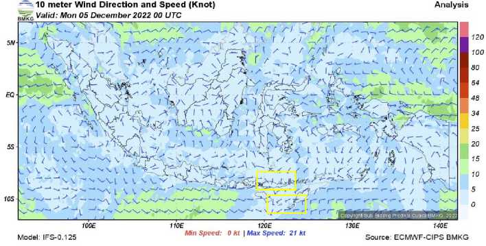
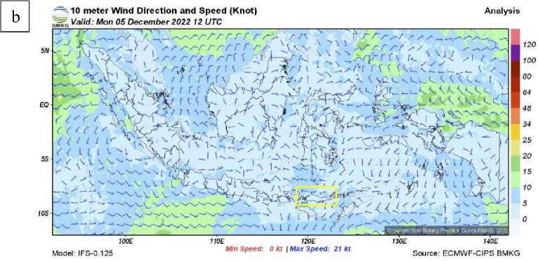
Figure 5.
Analysis of surface wind direction and speed on 5 December 2022 at (a) 00.00 UTC (08.00 WITA) and (b) 12.00 UTC (20.00 WITA).
Weather disturbances on the synoptic scale can change surface wind patterns, affecting surface current flow around the waters they pass through. Following an
analysis of the direction and speed of surface winds on 5 December 2022, the cyclonic circulation around the Arafura Sea has resulted in a change in the wind
flow. Surface winds around the Flores Sea at 00.00 UTC appear to be blowing from the south and turning westward in the western Flores Sea. Meanwhile, analysis at 12.00 UTC shows wind flowing from
the west to the east. This condition explains why on 5 December 2022, ocean surface currents in the Flores Sea moved in very varied directions.
a
b
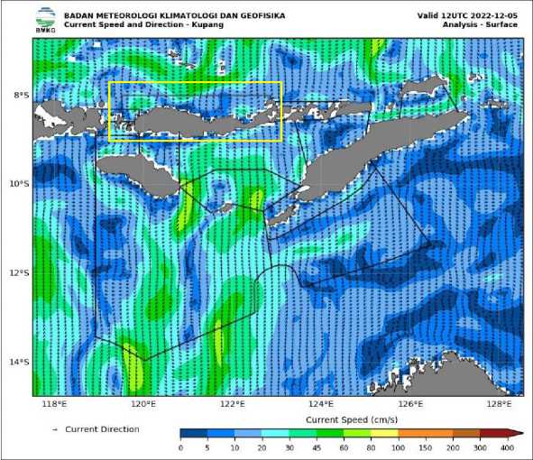
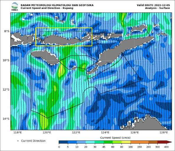
Figure 6.
Analysis of surface current speed and direction from BMKG OFS on 5 December 2022, at (a) 00.00 UTC (08.00 WITA) and (b) 12.00 UTC (20.00
WITA).
Comparing the Himawari-8 data with the BMKG OFS model (Figure 6), surface current movement appears to be directed differently. Estimated surface currents from Himawari-8 indicate that surface currents are dominant in the zonal direction following synoptic winds. However, the BMKG OFS model shows varying results in areas to the east and west of the Flores Sea dominated by zonal currents. The center, however, is dominated by meridional currents. Surface currents are not always influenced by synoptic wind. This can be due to differences in the input data. According to the Himawari-8 estimate, pixels in SST images are displaced by a simple concept. Using Wave Watch III, more complicated calculations are used that take into account factors such as bathymetry, wind, and others. It should also be noted, however, that sea level current data for Indonesia from BMKG OFS have not been validated. As such, it is important to be aware of the potential differences in input data when relying on surface current estimates, as this can significantly affect the accuracy of the final result.
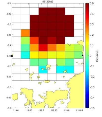
According to Figure 7, the bias error for the U component is generally greater than the bias error for the V component. North of the HF radar, the bias error varies between 0 and 0.5 ms-1, with the largest bias error occurring in the area farthest from the radar. The V component exhibits a different condition, where the bias error is smaller in the same area, with values ranging from -0.3 to 0.3 ms-1. Meanwhile, the U component in the area south of the HF radar location exhibits a lower bias error than in the area to the north, with values between -0.2 and 0.1 ms-1. Conditions in the V component are slightly different. There is a bias error of between -0.1 and 0.1 ms-1 associated with the V component in this area. Additionally, the bias error of the U component is slightly higher than that of
the V component in the area between LAWA and KARA radar HF. For components U and V, these values range from -0.1 to 0.2 ms-1 and -0.1 to 0.1 ms-1, respectively.
As shown in Figure 8, the RMSE of the U component is generally greater than that of the V component. There is a tendency for grids in the north areas of the HF radar to have a large RMSE of 0.5 ms-1 for the U component. RMSE values in the south area range between 0.1 and 0.2 ms-1. A similar situation can be observed for the V component, where most of the validation area, especially the northern area, shows a large RMSE with a value approaching 0.5 ms-1. In the southern area, the RMSE value is between 0.05 - 0.3 ms-1. Low RMSE values are found especially in the eastern area around KARA radar HF (within about 9.5 km).
Based on the bias and RMSE, a positive bias error indicates that ocean surface current estimation results are overestimated. Otherwise, a negative bias error indicates the opposite; the estimate is underestimated. At the same time, the RMSE shows the error level in the prediction results. The smaller the RMSE value (closer to 0), the more accurate the prediction results. On 5 December 2022 generally, the northern part of the HF radar range is chiefly overestimated, especially for the U component, while the values vary more for the V component. Areas with underestimated and overestimated estimates are not clustered together. They are scattered randomly and dominated by bias errors with values close to 0. The V component also indicates better RMSE. The RMSE for the U current component is also generally more extensive than that for the V current component. This means that the prediction error of surface current velocity for the V component is smaller than that for the U component. A combination of bias and RMSE indicates that the highest accuracy
for estimating ocean surface current speed is found in the area to the south. This is
U Current component BIAS
close to the HF radar location, especially for the V current component.
V Current component BIAS
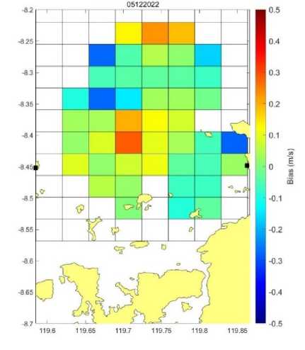

Figure 8.
Figure 7.
Bias error of the daily average of data every 20 minutes. Calculated for the U and V components on 5 December 2022 in the HF radar coverage area (black dots are HF radar point locations).
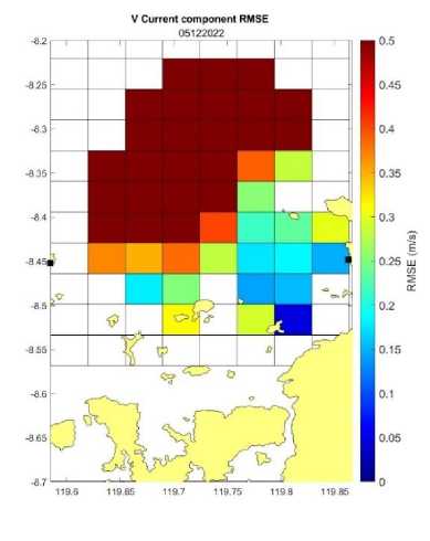
RMSE of the daily average of data every 20 minutes. Calculated for the U and V components on 5 December 2022 in the HF radar coverage area (black dots are HF radar point locations).
Daily average distributions of Flores Sea ocean surface currents observed from the Himawari-8 SST are dominated by east-west (zonal) currents. During the research period, surface currents varied more. This was due to synoptic weather disturbances, which resulted in a change in the direction of the Asian monsoon at that time. The resulting data has too high a speed as a result of the uncertainty in the calculations in the PIVLab used. This can lead to inaccurate results and should be addressed.
There is still a great deal of research to be done regarding the adjustment of PIV calculation methods such as interrogation windows, post-processing, etc., to produce better data accuracy estimations. In order to collect a better understanding of the quality of the estimated data produced, the addition of the research period is necessary.
REFERENCES
Balamurugan, R., & Jeeva, B. (2019).
Micron size particle image velocimetry by fast Fourier transform. 020156.
https://doi.org/10.1063/1.5130366
Bunea, F., She, Y., Ombao, H., Gongvatana, A., Devlin, K., &
Cohen, R. (2011). Penalized least squares regression methods and applications to neuroimaging.
NeuroImage, 55(4), 1519–1527.
https://doi.org/10.1016/j.neuroimage. 2010.12.028
Choi, J. M., Kim, W., Hong, T. T. M., & Park, Y. G. (2021). Derivation and
Evaluation of Satellite-Based Surface Current. Frontiers in Marine Science, 8.https://doi.org/10.3389/fmars. 2021.695780
Dabiri, D. (2006) ‘Cross-correlation digital particle image velocimetry—a review’, Turbulencia. ABCM, Curitiba, pp. 155–199.
Dorofeyev, V. L., & Sukhikh, L. I. (2019). Influence of surface currents on the nutrient fluxes from the shelf to the deep part of the Black Sea. Journal of Physics: Conference Series,
1359(1), 012074.
https://doi.org/10.1088/1742-6596/1359/1/012074
Frankignoul, C., Bonjean, F., & Reverdin, G. (1996). Interannual variability of surface currents in the tropical Pacific during 1987-1993. Journal of Geophysical Research: Oceans,
101(C2), 3629–3647.
https://doi.org/10.1029/95JC03439
Fujita, I., Muste, M., & Kruger, A. (1998). Large-scale particle image
velocimetry for flow analysis in hydraulic engineering applications. Journal of Hydraulic Research, 36(3), 397–414.
https://doi.org/10.1080/00221689809 498626
Ghalenoei, E., & Hasanlou, M. (2017). Monitoring of sea surface currents by using sea surface temperature and satellite altimetry data in the Caspian Sea Uav photogrammetry View project SAR Polarimetry Information Extraction View project Monitoring of sea surface currents by using sea surface temperature and satellite altimetry data in the Caspian Sea. Earth Observation and Geomatics Engineering, 1(1), 36–46.
https://doi.org/10.22059/eoge.2017.2 26309.1001
González-Haro, C., Isern-Fontanet, J., Tandeo, P., & Garello, R. (2020). Ocean Surface Currents
Reconstruction: Spectral
Characterization of the Transfer Function Between SST and SSH. Journal of Geophysical Research: Oceans, 125(10).
https://doi.org/10.1029/2019JC01595 8
Haryanto, Y. D., Riama, N. F., Purnama, D. R., Pradita, N., Ismah, S. F., Suryo, A. W., Fadli, M., Hananto, N. D., Li, S., & Susanto, R. D. (2021). Effect of Monsoon Phenomenon on Sea Surface Temperatures in Indonesian Throughflow Region and Southeast Indian Ocean. Journal of Southwest Jiaotong University,
56(6), 914–923.
https://doi.org/10.35741/issn.0258-2724.56.6.80
Havis, M. I., & Yunita, N. F. (2017). Surface Currents in Indonesian Sea Based on Ocean Surface Currents Near – Realtime (OSCAR) Data. Marine Technology for Sustainable Development, 27–31.
Hsu, T.-W., Shin, C.-Y., Ou, S.-H., & Li, Y.-T. (2011). Multi-Cross
Correlation Method in Particle Image Velocimetry. Journal of Mechanics, 27(3), 365–377.
https://doi.org/10.1017/jmech.2011.3 9
Nogueira, J., Lecuona, A., Ruiz-rivas, Rodriguez, P. A. (2002). Analysis and alternatives in two-dimensional multigrid particle image velocimetry methods: application of a dedicated weighting function and symmetric direct correlation. Measurement Science and Tchnology, 13, 963–974. https://doi.org/10.1088/0957-0233/13/7/302
Pastuchová, E., & Zákopčan, M. (2015). Comparison of Algorithms For Fitting a Gaussian Function Used in Testing Smart Sensors. Journal of Electrical Engineering, 66(3), 178– 181. https://doi.org/10.2478/jee-
2015-0029
Peng, Q., Xie, S.-P., Wang, D., Huang, R. X., Chen, G., Shu, Y., Shi, J.-R., & Liu, W. (2022). Surface warming– induced global acceleration of upper ocean currents. Science Advances, 8(16).
https://doi.org/10.1126/sciadv.abj839 4
Perkovic, D., Lippmann, T. C., & Frasier, S. J. (2009). Longshore Surface Currents Measured by Doppler Radar and Video PIV Techniques. IEEE Transactions on Geoscience and Remote Sensing, 47(8), 2787–2800. https://doi.org/10.1109/TGRS.2009.2 016556
Purba, N. P., Handyman, D. I. W., Pribadi, T. D., Syakti, A. D., Pranowo, W. S., Harvey, A., & Ihsan, Y. N. (2019). Marine debris in Indonesia: A review of research and status. Marine Pollution Bulletin, 146, 134–144.
https://doi.org/10.1016/j.marpolbul.2 019.05.057
Putriani, P. Y., Atmadipoera, A. S., & Nugroho, D. (2019). Interannual variability of Indonesian throughflow in the Flores Sea. IOP Conference Series: Earth and Environmental Science, 278(1), 012064.
https://doi.org/10.1088/1755-1315/278/1/012064
Raffel, M., Willert, C. E., Scarano, F., Kähler, C. J., Wereley, S. T., &
Kompenhans, J. (2018). Particle Image Velocimetry. Springer
International Publishing.
https://doi.org/10.1007/978-3-319-68852-7
Rio, M.-H., Santoleri, R., Bourdalle-Badie, R., Griffa, A., Piterbarg, L., & Taburet, G. (2016). Improving the Altimeter-Derived Surface Currents Using High-Resolution Sea Surface Temperature Data: A Feasability Study Based on Model Outputs. Journal of Atmospheric and Oceanic Technology, 33(12), 2769–2784.
https://doi.org/10.1175/JTECH-D-16-0017.1
Russmeier, N., Hahn, A., & Zielinski, O. (2017). Ocean surface water currents by large-scale particle image velocimetry technique. OCEANS 2017 - Aberdeen, 2017-October, 1– 10.
https://doi.org/10.1109/OCEANSE.2 017.8084843
Supriyadi, E., Hidayat, R., Santikayasa, P., & Ramdhani, A. (2021). An
Analysis of Surface Ocean Currents from HF Radar Measurements in the Bali Strait and the Flores Sea, Indonesia. International Journal on
Advanced Science, Engineering and Information Technology, 11(4).
Thielicke, W., & Stamhuis, E. J. (2014). PIVlab – Towards User-friendly, Affordable and Accurate Digital Particle Image Velocimetry in
MATLAB. Journal of Open Research Software, 2.
https://doi.org/10.5334/jors.bl
Wichmann, D., Delandmeter, P., &
Sebille, E. van. (2019). Influence of Near‐Surface Currents on the Global Dispersal of Marine Microplastic. Journal of Geophysical Research: Oceans, 124(8), 6086–6096.
https://doi.org/10.1029/2019JC01532 8
Yang, M., Guan, L., Beggs, H., Morgan, N., Kurihara, Y., & Kachi, M.
(2020). Comparison of Himawari-8 AHI SST with Shipboard Skin SST Measurements in the Australian Region. Remote Sensing, 12(8),
1237.
https://doi.org/10.3390/rs12081237
ECOTROPHIC • 17(2): 253-267 p-ISSN:1907-5626,e-ISSN: 2503-3395
267
Discussion and feedback