OIL SPILL SIMULATION IN THE BALI STRAIT USING THE GNOME AND FVCOM MODELS ON EASTERLY SEASON
on
Oil Spill Simulation in The Bali Strait Using the GNOME...,[Pande Putu Hadi Wiguna, dkk]
OIL SPILL SIMULATION IN THE BALI STRAIT USING THE GNOME AND FVCOM MODELS ON EASTERLY SEASON
Pande Putu Hadi Wiguna1*), I Gede Hendrawan2), Takahiro Osawa3)
1)Indonesian Agency for Meteorlogical Climatological and Geophysical (BMKG). 2)Departement of Marine Sciences, Faculty of Marine Science and Fisheries, Udayana University, Denpasar, Bali, Indonesia.
3)Center of Research and Application of Satellite Remote Sensing (YUCRAS), Yamaguchi University, Ube-shi Yamaguchi Japan.
*Email: greenearthcadet@gmail.com
ABSTRACT
Among several forms of marine pollution, oil damages coastal ecosystems. Repeated reports of oil contamination in the marine environment can partly load with major shipping lines. The Ketapang-Gilimanuk crossing over the Bali Strait is Indonesia's second busiest ferry port after Merak-Bakauheni. The most congested shipping routes can carry a significant risk of environmental damage from an oil spill. Oil spill trajectory modelling is carried out to reduce the impact of this possible disaster. Therefore, the use of modelling to ascertain the route of the oil spill was considered. The oil leak path is simulated using the GNOME model. Two oil spill scenarios were used as input models. The chosen location is around the Ketapang Gilimanuk crossing, as well as the time of the easterly season. An ocean HF radar stationed in the Bali Strait verifies the accuracy of the current marine data generated by FVCOM. To see the pattern of the oil spill trajectory based on a ten days simulation, we combined the latest data from FVCOM with GNOME. To determine the ability of the model to predict the flow and trajectory of oil spills in the Bali Strait, this study try to analyze and interpret the oil spill trajectory from model and then validate the model results with satellite imagery.
Keywords: Bali strait; oil spill; trajectory; GNOME; FVCOM; HF Radar
A significant amount of ocean pollution comes from oil. Each year, 380 million gallons of oil are released into the waters by anthropogenic and natural activities (Pisano et al., 2016). (El-Magd et al., 2020; Fingas & Fingas, 2002) About 48% of oil spills occur due to crossing ships, 29% from crude oil mining, and only 5% from tanker accidents.
A number of oil-contaminated marine environments can be attributed to the main shipping lanes (Brekke & Solberg, 2005). Ketapang-Gilimanuk is Indonesia's second busiest ferry crossing route after
Bakauheni-Lampung (Pricilia, 2018). Around 6 million people will cross this crossing route between Java and Bali in 2018-2020 (BPS Banyuwangi, 2022). Thus, the movement of numerous ships in crowded areas took place. With heavy crossings, oil spills are more likely to occur. Oil spill risk increases with heavy crossings (Putra et al., 2021). As a result of ship crossing activity, there is a potential oil spill.
To mitigate this potential disaster, oil spill distribution is modeled. It is crucial to understand where an oil spill will move and what impact it will have on the environment (Amir-Heidari & Raie, 2019).
As mitigation efforts from the incident progress, it will be important to know how the oil spill will distribute. A particle's movement can be determined through direct observation or numerical hydrodynamic modelling (Huang et al., 2008). Direct observation requires significant effort, time, and money (Putra et al., 2020).
Since wind and current generate oil spill movement, modeling is used to determine the direction of spill distribution (Tri Rezki et al., 2018). The GNOME (General NOAA Operational Modeling Environment) model (Zelenke et al., 2012) was used to simulate the oil spill's track because of its high predictive accuracy ((Farzingohar et al., 2011; Balogun et al., 2021; Chang et al., 2011). An oil spill trajectory model GNOME depends on input force. It is estimated that wind direction and speed influence oil spills by 3% (Hyder et al., 2017; Prasad et al., 2020; Tri Rezki et al., 2018). One of the numerical hydrodynamic models developed by several parties is the Finite Volume Coastal Ocean Model (FVCOM). Its spatial coverage is better with satellite-derived ocean currents. A relatively low spatial resolution and retrieval technique assumptions constrain them. Because the ocean is chaotic and measurements are scarce, numerical simulations of threedimensional ocean currents with high spatial and temporal resolution may contain small-scale features not present in the real ocean or dislocated in space and time (Sperrevik et al., 2017). This research uses the FVCOM model to generate ocean current data. In situ observation of BMKG (Indonesian Agency for Meteorological, Climatological and Geophysics) HF (High
Frequency) Radar Ocean Current in Ketapang validates the output data of the FVCOM model before coupling it with GNOME trajectory. Using the captured image of Sentinel-1, which matches a backscatter value indicated as an oil spill (Nugroho et al., 2021; Puspitasari et al., 2020), is used to pinpoint the location of the oil spill. Also, other scenarios (NOAA (National Oceanic and Atmospheric Administration) - Office of Response and Restoration, 2016) were developed to cover oil spill trajectory during easterly seasons.
The potential for catastrophic ocean pollution is assessed using simulations and models of how pollutants move. A contingency planning system is required to run an oil spill modeling simulation (Fuad, 2021). There are no studies that discuss the potential and modeling of oil spills in the Bali Strait, there for, this study is expected to determine the ability of the model to predict the flow and trajectory of oil spills in the Bali Strait.
The 80km long Bali Strait connects the Java Sea north to the Indian Ocean south. Approximately 60km wide and 365m deep in the south, the strait narrows to the north (2km wide and 50m deep) (Hanifa et al., 2020). Approximately 137 km2 of research area is located at -8.3062517 Latitude and 114.5543985 Longitude. Several complicated operations take place in the Bali Strait, including fishing, tourism, and people and goods movement.
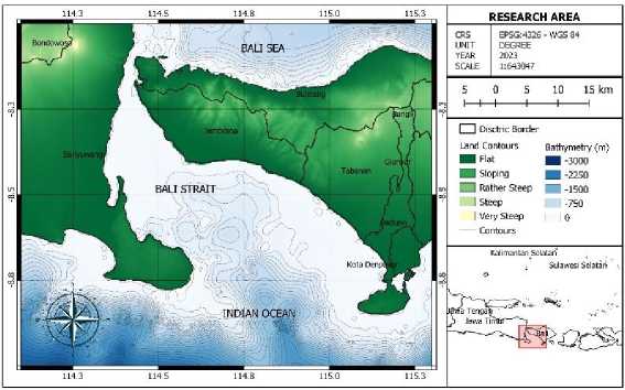
Figure 1.
Research Area
Brekke and Solberg, (2005) In their research, 45% of oil pollution is caused by ship operative discharge, and Putra, Osawa and Astawa Karang, (2021) found oil spill risks increase with heavy crossing activity, making the Bali Strait susceptible to oil spills as well. This method uses Sentinel-1 satellites that detect oil spill backscatter and the location of Ketapang-Gilimanuk ferry crossings. The case studied are July as followed by Easterly season. As noted by (Supriyadi et al., 2021), the current velocity in the Bali Strait is higher in June, July, and August where these three months are included in the easterly season in Indonesia. This timing aims to see more dynamic oil movements, because the flow is faster. Apart from that, choosing the time during the Easter season or dry season also aims to minimize the occurrence of ”look-alike” slicks, the oil-free false targets because of rain cells and others (Carvalho et al., 2021).
GNOME can download for free at https://response.restoration.noaa.gov/oil-and-chemical-spills/oil-spills/response-tools/downloading-installing- and-
running-gnome.html. Input parameters for this model include sea currents
generated by the FVCOM model. The following data inputs are required for generation of current sea data in FVCOM.
-
• Geospatial Information Agency (BIG) bathymetry data with a resolution of 180 m. Available at
https://tanahair.indonesia.gi.id.
-
• From Tide Model Driver (TMD): M2, S2, N2, K2, K1, O1, P1, Q1, MM, MF, M4, MN4, MS4, 2N2, S1, 2Q1, J1, L2, M3, MU2, NU2, and OO1.
-
• Ketapang and Gilimanuk water levels are from BMKG AWS (Automatic Weather Station) 2021-2022.
-
• Wind directions and speeds are obtained from ECMWF (European Centre for Medium-Range Weather Forecasts) , available at
https://www.ecmwf.int/en/forecasts/d atasets.
-
• Sentinel-1A SAR (Satellite Aperture Radar) satellite data was downloaded via the Copernicus Open Access Hub web, https://scihub.copernicus.eu/.
-
• High Frequency (HF) radar in Bali Strait obtained from BMKG.
-
2.3 Data Processing
-
2.3.1 Validating the Tide Elevation with BMKG AWS Water Level Data
-
To generate ocean currents data in FVCOM hydrostatic modeling, tidal elevation is one of the input data. It is necessary to verify the suitability of the data from the TMD (Tidal Model Driver) by comparing it with the observation data. TMD model data will be verified with observation water level data from BMKG AWS (Automatic Weather Station) which located at Ketapang and Gilimanuk ports. RMSE (Root Mean Square Error) and correlation analysis were performed, as shown in equations (1) and (2):
∑χy-(^≡
J(∑^-∑^j(∑^∑f)
RMSE
∖ ∑ I = 1 (Xinsitu,i ^model, j )
N n
(2)
This equation represents the correlation coefficient, n represents the amount of data, x represents the observation on the field, in this case Water Level Data from BMKG AWS (, and y represents the model, in this case TMD data. An RMSE equation is based
on the observations, X model on the model findings, and n on the observations.
The use of RMSE refers to previous research on tidal data and Correlation values are used as an initial detection of the relationship between the model and predictions. It is assumed that if correlation is good, then the other validation methods that will be applied to the data will be related to each other. Correlation is defined to determine the relationship between 2 variables, it is not stated whether the 2 variables are different or not.
-
2.3.2 Generate the Sea Surface Current Data from
Hydrodynamic Model
GNOME model needs wind and sea current data for universal movers that move oil in the water (Fuad, 2021). Current movement patterns are obtained through simulations using the Finite Volume Coastal Ocean Model (FVCOM). A model warm up period of one month is allowed before the model configuration date to allow for a longer period of initial conditions. Figure 2 shows the domain model area, adjusted for Bali Strait, the research location and Table 1 shows parameter specifications and notes.
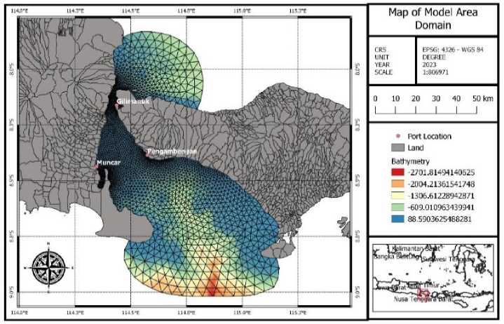
Figure 2.
Model Area Domain
Table 1. Input and settings of the FVCOM model used in this research
|
Item |
Information |
|
Grid |
Unstructured triangular grid with a resolution of 300m - 5000m (distance between the two closest nodes) |
|
Layer Tidal components |
Parabolic layer with fourth sigma layer Tide Elevation (M2, S2, N2, K2, K1, O1, P1, Q1, MM, MF, M4, MN4, MS4, 2N2, S1, 2Q1, J1, L2, M3, MU2, NU2, and OO1) are got from Tide Model Driver (TMD) |
|
Wind |
ERA5 Wind data from 2011-2020 are obtained from European Centre for Medium-range Weather Forecast (ECMWF). This data came with 0.125 degrees of spatial resolution. |
|
Bathymetry |
Batimetri Nasional (BATNAS) from Badan Informasi Geospatial (BIG) with resolution 180m. |
|
Time simulation Timestep |
1 – 31 July 2020 10 second |
-
2.3.3 Verification of the FVCOM output with BMKG High Frequency (HF) Radar
BMKG HF Radar data are used to validate the output data from FVCOM to
ensure accuracy. This model will be validated with observations from BMKG HF Radar in 01-31 July. Figure 4.3 shows where observation points will be placed for current verification.
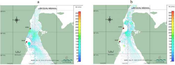
Figure 3.
HF Radar radial velocity: a. BOOM site, b. WARU site (Supriyadi et al., 2021).
There are five variables in HF radar
data, including longitude, latitude, zonal current, meridional current, and time, with a spatial resolution of 0.0045 degrees or 500 meters.
Grid conversion takes place before comparing model data with observation data from the HF Radar. In contrast to the
FVCOM grid, which uses a triangular grid, the HF Radar grid uses a rectangular grid. Sea current data are read from FVCOM
and a grid is created identical to the observation data grid from HF Radar. In addition, natural neighbor interpolation was performed on the sea current data model. Statistics such as correlation and Willmott's Formula are used to evaluate
the accuracy of model-observed sea
surface currents.
∑χy- (∑ Ξ )(∑ y)
√(∑ χ2~ (∑ I ) - )(∑y2- (∑ I ) - )
=
∑i=ι |Pj-Qj|
1- ∑i=ι |Ol- ̅| ∑ i=ι |Qj-̅|
∑i=ι |Pj-Oj|-1
Jika ∑P=I | Pi - ot|≤c∑ ^l
Jika ∑P=I | Pt - ot|>c∑P=I
(3)
_
| Ot - ̅|
_
| Ot - ̅|
(4)
In equation (3), r represents the correlation coefficient, n represents the amount of data, x represents the value of the observation on the field, in this case, HF Radar, and y represents the value of the model, in this case, FVCOM.
Calculating Willmott formulas involves finding the difference between prediction models and observations. This is related to the number/relative average
value of observations from the exact model. An accurate model has a Willmott formula of 1 or 1. It also includes observation deviation compared to the mean observed value. In equation (4), Pi is the value obtained from the model, Oi is the observed value, ̅ is the average observed value and c is equal to 2, which represents the average absolute deviation obtained from the equation in the study Willmott et al., 2012. The range of correlation and Willmott index values can be categorized as follows: 0.9 – 1 is very good; 0.7 – 0.9 is good; 0.5 – 0.7 is moderate; 0.3 – 0.5 is bad; 0 – 0.3 is very bad.
-
2.3.3 Verification of the FVCOM output with BMKG High Frequency (HF) Radar
It was decided to create oil spill scenarios at two locations and at two different times, namely Ketapang-Gilimanuk ferry crossing. 45% of oil pollution at sea can be attributed to ship operative discharge (Brekke & Solberg, 2005). According to I. E. H. Putra et al., 2021, oil spills can occur where there is heavy crossing activity. Another way is to use Sentinel-1 SAR satellite data as an indicator. To describe the eastern season July 2020 were selected. June, July, and August are the east monsoon months in Bali Strait that have higher current velocities. According to Sentinel-1, a spot near the Ketapang-Gilimanuk crossing on 16 July 2020 was detected. this make the
scenario 3A initial location is based on satellite detection.
As a result of NOAA’s Office of Response and Restoration (2016), calculations are based on the approach method. For non-tank vessels, the worstcase discharge is defined as 10% of their fuel capacity. An average tugboat can carry 1500-25000 gallons of oil, according to NOAA - Office of Response and Restoration, 2016. Vessel Finder, 2022, estimated that this ferry will carry 9000019000 gallons of fuel. It is dominated by ferry crossing activities between Ketapang and Gilimanuk. Between 9000 and 19000 gallons is the most dangerous spill. It is simulated on the fourth day or the day that Sentinel detects a potential oil spill one month before the spin-up model period in January and July. Due to the limitations of oil-spill modeling and the unpredictability of clean-up operations, simulations could only run for ten days (Barker et al., 2020; Huynh et al., 2021).
The sea current data from FVCOM model is verified with HF radar and the GNOME model is coupled with sea current data from FVCOM. Oil spill modelling results are interpreted with GNOME software. GNOME uses four inputs; maps in .bna format, wind data from ECMWF, sea current data from the
FVCOM hydrodynamic model, and an oil spill scenario.
To create the map, the GNOME output will be processed into QGIS software. Based on (Galt, 1996), ”minimum regret” analyzes the sensitivity of different estimates to errors in input data as well as evaluating possible alternate scenarios. During model setup, the ”what if” function can improve the model’s prediction accuracy by accounting for environmental uncertainties and errors (Engha Isah & Anifowose, 2021; Korsah & Anifowose, 2014). Therefore, the ”red splots” function of GNOME was engaged (Cheng et al., 2011), and spill scenarios were developed using the hydrodynamic data of Table 1.
The next step is to detect oil spills by applying the adaptive threshold method using the Oil Spill Detection Tools in the SNAP (Sentinel Application Platform). Then proceed with the Geometric Calibration process to apply Ellipsoid Correction. This is so that the image position is not inverted and in accordance with the field conditions. The last step is to convert dB to get clear image results before performing a profile plot analysis on the dark area. This is used as the area suspected of an oil spill. The plot profile results will be validated in table 2.
Table 2. Classification of Oil Spill Thickness according(Sun et al., 2016)
Plot Value (dB) Thickness (µm) Oil Type
-
- 15 – (-20) ≤ 50 Diesel
-
- 20 – (-25) 50-200 Light Crude Oil
-
- 25 – (-30) 200-1200 Medium Crude Oil
In order to estimate wind speed around Sentinel-1A, different treatments are applied. Detection of oil spills on radar images depends on the wind speed at the time. Low wind speeds do not produce backscatter because capillary and gravity
waves do not form, resulting in dark areas that resemble oil spills (Jaelani, 2021). In contrast, oil spilled on the sea surface will mix with seawater at high winds and sink to the bottom of the ocean. This will prevent them from being detected on radar
images (Jaelani, 2021; Topouzelis, 2008). Before do the Wind Field Estimation, we do need to preprocessing and calibration the Sentinel-1A data. Sentinel Application Platform (SNAP) provides the tools for calibrating Level 1 (L1) ground range detected (GRD) Sentinel-1 data products in order to obtain the Normalized Radar Cross Section (NRCS) values, known as Sigma0, that are used for calculating wind speed. SNAP preprocessing steps on L1-GRD data include orbit correction, thermal noise removal, radiometric calibration (to calculate Sigma0), land masking, and multi-looking to smooth out speckle noise (James, 2017).
Wind can affect the backscatter displayed by radar imagery. For this reason, wind estimation around the oil spill area is carried out. SNAP also provides a Wind Field Estimation Tool. This tool applied the model function CMOD5 (The C-band geophysical model function, CMOD5, is developed by ECMWF and KNMI for use with the ERS and ASCAT scatterometers). The CMOD5 function relates Sigma0 from copolarised (vertically polarised transmit and receive known as VV) C-band SAR data to wind speed, wind direction and SAR incidence angle. A look up table is created by using CMOD5 to calculate Sigma0 for a range of wind speeds, relative wind directions and incidence angles (James, 2017). The CMOD functions for VV polarization wind speed estimation is described in equation (5).
CT ∘ VV=А[1+bi ×cos ∅+b2 × cos 2∅]b (5)
Where σ◦ vv is the VV-polarization of NRCS for sea surface, ∅ is the direction of wind relative to radar look, exponent of B is a fixed value and coefficients A, b1 and b2 are described as a function of wind speed V (Naz et al., 2021). After get the result from Wind Field Estimation on SNAP, validation with previous research criteria, oil spills can be detected with wind speeds between 2 and 14 m/s (Prastyani & Basith, 2019) and A high level of confidence has a wind speed of 610 m/s. While data that has a wind speed of 3-6 m/s is data with a medium level of confidence (Indregard et al., 2004) are applied to distinguish which dark areas are caused by oil spills or just look-alikes.
-
3. RESULTS AND DISCUSSION
-
3.1 Validating the Tide Elevation
-
(TMD)
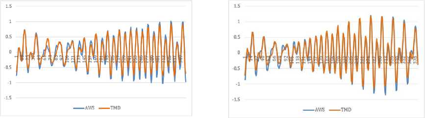
Observation data for both AWS Ketapang and Gilimanuk were only installed in early 2020 and required several periods to produce stable data. So, this study using AWS data for 1 year from November 2021 to October 2022. Figure 4(a) compares TMD results (blue line) and water level observations (orange line) at Ketapang Port, Banyuwangi. It can be seen that the graphic pattern of the two data is almost the same. It's just that the TMD data looks slightly overestimated than the AWS observation data. Figure 4(a) produces a correlation value of 0.969 and an RMSE of 0.007 m. This value shows a very significant correlation between the model and field observations at Ketapang Port, Banyuwangi.
(a) (b)
Figure 4.
(a) AWS Water Level Vs Tidal Model Driver (TMD) in Ketapang Area; (b) AWS Water Level Vs Tidal Model Driver (TMD) in Gilimanuk Area
Figure 4(b) compares TMD (blue line) and water level observations (orange line) at Gilimanuk Port, Bali. Overall, the TMD pattern describes the pattern of field observations well, as can be seen from the very precise graphic form between two. Graph 5.2 produces a correlation value of 0.970 and an RMSE of 0.012 m. These two values show a verytrong relationship and value between the model and observations at Gilimanuk Harbor, Bali.
-
3.2 Validation of the FVCOM output with BMKG High Frequency (HF) Radar
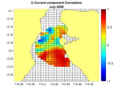
July 2020 was chosen to describe the sea current state during the easterly season. Figure 5. (a) is a correlation graph
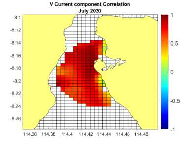
of the U-directed Current Component in July 2020. A large portion of the validation area, especially in the southern validation area, has a value of 0.5 or higher. While in the northern validation area, it has a lower correlation value, between 0.5 and -0.5. This correlation value indicates poor relationship between variables in the northern validation area. Meanwhile, negative values indicate an opposite relationship between the model U component variables and the observed U component variables. From the validation of these two current components, it can be seen that the V current component in the model can describe the condition of the V current component in the field.
(a) (b)
-
Figure 5.
-
(a) U Current Component Correlation July 2020; (b) V Current Component Correlation July 2020.
(a) (b)
-
Figure 6
-
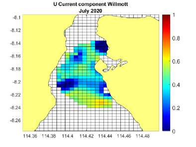
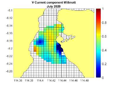
(a) U Current Component Willmott July 2020; (b) V Current Component Willmott July
2020.
Figure 6 shows the spatial depiction of the Willmott index values between the
U and V components produced by the model and observations. Figure 6 (a) shows the spatial values of the U component Willmott index. In general, the Willmott index values range from 0 – 0.6 are more in the mid to north validation area. In contrast, the Willmott index
between 0 and 0.7 is more in the area of southern validation. This shows that the model describes the field situation well in the southern validation area. Meanwhile, in the central and northern parts, the model depiction tends to be good or bad. For the Willmott index component V as illustrated in Figure 6 (b), it can be seen that the range of Willmott index values is
between 0-0.8, with the distribution of
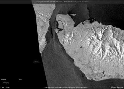
Figure 7.
index values from 0.5 to 0.8 evenly distributed from the north, center, and to
the south. This shows that the model description of the current V component can be done well.
-
3.3 Initial Location for Ketapang-Gilimanuk Scenario 3A - 16 July 2020
On 16 July 2020, a suspect was detected for the first time. It is necessary to re-process using SNAP software and treatment as described in the previous chapter. Shown in the red circle area is the area suspected of an oil spill. The location is located at the Ketapang - Gilimanuk Ferry crossing.
Oil Spill Suspect Area at Ketapang-Gilimanuk Harbour, 16 July 2020
(a) (b)
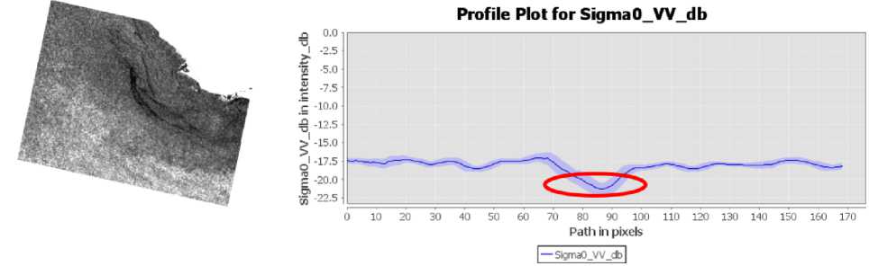
Figure 8.
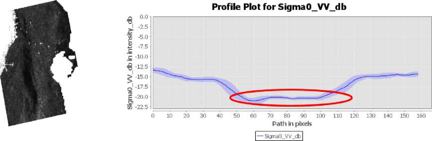
(a) Result from Oil Spill Detection Tools on 16 July 2020.; (b) Profile Plot VV Chanel on 16 July 2020
To ensure that the suspected oil leak is an oil spill, further analysis was conducted on the Sentinel-1A catch. Using the adaptive threshold and Oil Spill Detection Tools contained in the SNAP application, the results are shown in Figure 5.19. Figure 8 (a) is the result of the Oil Spill Detection Tools where a black area is seen as a suspect of the presence of an oil spill in the waters of the Bali Strait. It extending from north to south, cutting across the Bali Strait crossing. Figure 8 (b) is the result of profile plot from channel VV image Sentinel-1A, where the dark area suspected of an oil spill has plot value between -17-(-21) db, which is
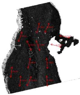
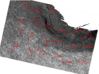
approximately -3.5-(-4) db lower than the amplitude around. Wind speed data were obtained from Sentinel 1A images which were processed using the wind prediction tools available in the SNAP application. From the wind analysis results in Figure 9, the average speed for the area is around 4.6 m/s. In a study by Indregard, et al (2004) who studied benchmarking oilspil recognition approaches, to determine the level of confidence, wind speed data is the determining factor. Data that has a wind speed of 3-6 m/s is data with a medium level of confidence. According to this study, the mean value of 4.6 m/s fits with medium confidence.
(a)
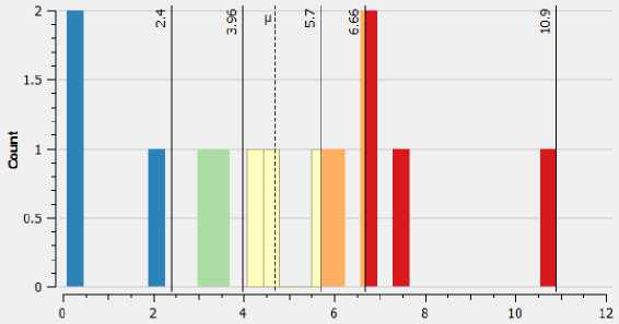
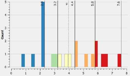
Figure 9
(b)
-
(a) Wind estimation around oil spill area the Wind Speed Estimation Tools from the SNAP application on 16 July 2020.; (b) The histogram spread of wind speed data from wind speed estimation
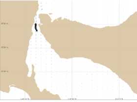
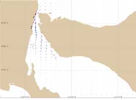
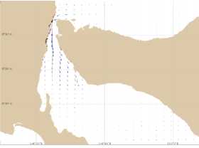
This simulation simulates the distribution pattern of oil spills in the Bali Strait during the Timuran season. We represent July in this simulation, as the eastern season begins in June, July and August. Sentinel 1A satellite imagery provides the initial oil spill area in this scenario. The satellite captured a dark area suspected of an oil spill near the Ketapang-Gilimanuk crossing. Based on the captured image, the spill shape and location were determined. According to satellite data, the spilled oil covered 2,897 km2 and had a North-South shape.
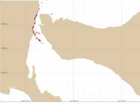
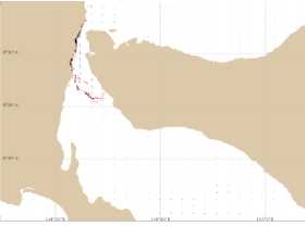
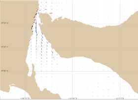
As the oil spill approached the coast of Java 24 hours after the first simulation was run, 380 gallons (2%) are moored near Watudodol. In the water between Watudodol, Ketapang, and Boom Beach, 11928 gallons (62.8%) are still floating. 6686 gallons (35.2%) have evaporated and dispersed and there is no oil left. After 48 hours, the oil spill spread to Kampe beach in Java and Candikusuma Beach in Bali. The spread of oil has accelerated 72 hours after it was discovered. The oil spill is estimated to have moored 1064 gallons (5.6%), with 6059 gallons (31.9%) still floating in the waters, especially south of the first location. It is estimated that 11,681 gallons (61.5%) of oil have evaporated and dispersed, and 190 gallons (1%) have left the study area. The oil is moving southeast-south toward Candikusuma waters. It is estimated that in the following days, the area of distribution of the oil spill will expand, and in the next 120 hours, even though 74.9% or 14226 gallons of oil has evaporated and dispersed, 3875 gallons (20.4%) remain in the water. In Bali, its
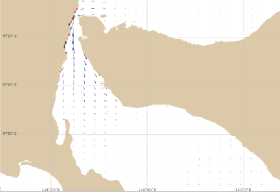
distribution area begins to approach Pengambengan. On 24 July 2020 or 192 hours after the first spill was detected, the oil spill has reached a radius of 40.9 km. The coast of Java, such as Watudodol, Ketapang, and Boom beach, is estimated to have the most oil spills. Some of them are moored near Candikusuma beach on Bali, while others are found in Pengambengan waters.
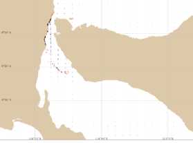
240 hours after the spill was discovered, 16182 gallons (85.2%) are estimated to have evaporated and dispersed, while 2108 gallons are still floating scattered across Cacalan beach, Boom beach, Santen island, Cemara Gading beach, Cungkingan beach, Pafruit beach, and Candikusuma beach. A total of 494 gallons (2.6%) are moored on the beach, most of which are near Ketapang and Watudodol. Another 209 gallons (1.1%) are outside the study region.
As a result of the Sentinel 1A satellite's detection of black areas suspected to be oil spills, we used the GNOME model to conduct scenario. Due to past events and the lack of evidence in mass media reports, the oil spill was difficult to validate. It was considered that satellite imagery was available for approximately eight to nine days between when it was discovered and before or after it was discovered. Note that the quality of satellite catches at the time, which is heavily affected by weather conditions, can also make it difficult to verify oil presence as simulated in the GNOME model.
00

24
48
72
96

120

144
168
192
216
240
Figure 10.
Oil Spill simulation from Scenario 3A in every 24 Hour
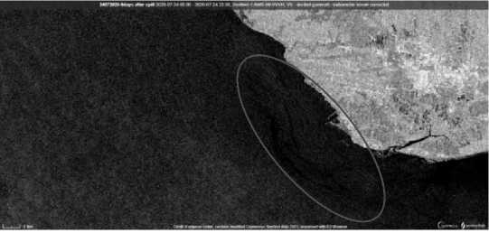
Figure 11.
Oil Spill Suspect Area near the Pengambengan Fishing Port – 24 July 2020
(a) (b)
Figure 12.
(a) Result from Oil Spill Detection Tools on 24 July 2020.; (b) Profile Plot VV Chanel on 24 July 2020
(a)
(b) Figure 13.
-
(a) Wind estimation around oil spill area the Wind Speed Estimation Tools from the SNAP application on 24 July 2020.; (b) The histogram spread of wind speed data from wind speed estimation
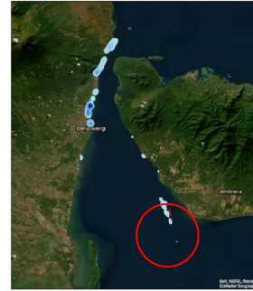
With Sentinel 1A satellite imagery, scenario 3A, or July 16, 2020, the GNOME trajectory model has been successfully validated. Eight days after the incident, an image showing a black area led to suspicion that an oil spill occurred. To make the task easier, the SNAP application uses an adaptive threshold and Oil Spill Detection Tools to identify suspected oil spill areas in Sentinel 1A imagery.
Figure 12 (a) shows an area that has undergone adaptive threshold treatment. There is a suspected oil spill in the dark area, which has a amplitude of around 17.5-21.5 db. This value is approximately 3-3.5 db
lower than the surrounding waters amplitude. From the wind estimation results in Figure 13, the average speed for the area is approximately 3.9 m/s. At the confidence level classification by Indregard, Solberg and Clayton (2004), 4.3 m/s is medium confidence. The GNOME model was used to determine whether an oil spill was floating around Pengambengan waters during that time. Image 15 (b) is produced by comparing the model results to the red satellite captured image 15 (a). As a result of satellite imagery capture, the simulation results are similar to the actual situation in the field.
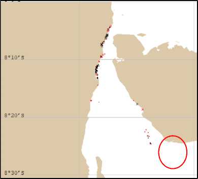
Figure 14.
GNOME model result in 24 July 2020 or day 8 after the first oil spill detected
(a) (b)
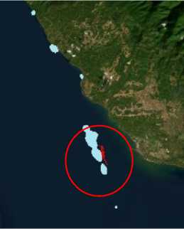
-
Figure 15.
Matching between GNOME result with Sentinel 1A Capture in 24 July 2020
As a result of limited data, it is difficult to validate the GNOME oil spill model. Media coverage of the oil spill in the Bali Strait is virtually impossible to find both online and in print. Satellite imagery was used to validate the GNOME model. Nugroho et al., 2021 also used satellite imagery to test the GNOME model oil spill trajectory. The distance between the first and second fastest captures in this study was July 16 2020, and the distance between the first and second fastest captures was July 24 2020. It took eight days for a second capture to occur in this study. According to Fingas & Brown, 2017, the long acquisition time made it difficult to detect oil spills.
Based on the favorable results of FVCOM data validation on HF Radar observations in the Bali Strait at easterly season, it is evident that FVCOM can provide accurate flow data for the oil spill trajectory model. GNOME trajectory results supported by FVCOM flow data can produce quite accurate predictions based on validation result from Sentinel 1A oil spill detection.
Despite the fact that there is no news in print or electronic media regarding oil spills, there is a need for further research with respect to the prediction of oil spill patterns at more specific times. In addition, satellite imagery can be used as a validation method if there has been no news in print or electronic media regarding an oil spill of any significance.
REFERENCES
Amir-Heidari, P., & Raie, M. (2019). A new stochastic oil spill risk assessment model for Persian Gulf: Development, application and evaluation. Marine Pollution Bulletin, 145, 357–369.
Balogun, A.-L., Yekeen, S. T., Pradhan, B., & Wan Yusof, K. B. (2021). Oil spill trajectory modelling and
environmental vulnerability mapping using GNOME model and GIS. Environmental Pollution, 268, 115812. https://doi.org/https://doi.org/10.1016/j .envpol.2020.115812
Barker, C. H., Kourafalou, V. H., Beegle-Krause, C. J., Boufadel, M., Bourassa, M. A., Buschang, S. G., Androulidakis, Y., Chassignet, E. P., Dagestad, K.-F., & Danmeier, D. G. (2020). Progress in operational modeling in support of oil spill response. Journal of Marine Science and Engineering, 8(9), 668.
BPS Banyuwangi. (2022, July 6). Produksi Angkutan Penyeberangan Gilimanuk. BPS Banyuwangi.
https://banyuwangikab.bps.go.id/statict able/2015/02/02/84/produksi-angkutan-penyeberangan-gilimanuk-2011-2021.html
Brekke, C., & Solberg, A. H. S. (2005). Oil spill detection by satellite remote sensing. In Remote Sensing of Environment (Vol. 95, Issue 1, pp. 1– 13).
https://doi.org/10.1016/j.rse.2004.11.0 15
Carvalho, G. de A., Minnett, P. J., Ebecken, N. F. F., & Landau, L. (2021). Oil Spills or Look-Alikes? Classification Rank of Surface Ocean Slick Signatures in Satellite Data. Remote Sensing, 13(17).
https://doi.org/10.3390/rs13173466
Chang, Y.-L., Oey, L., Xu, F.-H., Lu, H.-F., & Fujisaki, A. (2011). 2010 oil spill: trajectory projections based on ensemble drifter analyses. Ocean Dynamics, 61(6), 829–839.
Cheng, Y., Li, X., Xu, Q., Garcia-Pineda, O., Andersen, O. B., & Pichel, W. G. (2011). SAR observation and model tracking of an oil spill event in coastal waters. Marine Pollution Bulletin,
62(2).
https://doi.org/10.1016/j.marpolbul.20 10.10.005
El-Magd, I. A., Zakzouk, M., Abdulaziz, A. M., & Ali, E. M. (2020). The
potentiality of operational mapping of oil pollution in the mediterranean sea near the entrance of the suez canal using sentinel-1 SAR data. Remote Sensing, 12(8).
https://doi.org/10.3390/RS12081352
Engha Isah, M., & Anifowose, B. (2021). An Analysis of the Fate and Trajectory Simulation of Bonny Light Crude From The Dangote Single Point Mooring(SPM) Terminal Off the South Atlantic Ocean, Lagos Nigeria. International Oil Spill Conference Proceedings, 2021(1), 689260.
https://doi.org/10.7901/2169-3358-2021.1.689260
Fingas, M., & Brown, C. (2017). A Review of Oil Spill Remote Sensing. Sensors, 18, 91.
https://doi.org/10.3390/s18010091
Fingas, M., & Fingas, M. (2002). The
Basics of Oil Spill Cleanup. In The Basics of Oil Spill Cleanup.
https://doi.org/10.1201/978142003259 8
Fuad, M. A. Z. (2021). OIL SPILL TRAJECTORY SIMULATION AND ENVIRONMENTAL SENSITIVITY INDEX MAPPING: A CASE STUDY OF TANJUNG PRIOK, JAKARTA. Journal of Environmental Engineering and Sustainable Technology, 8(2), 47– 54.
Galt, J. A. (1996). Digital distribution standard for NOAA trajectory analysis information.
Hanifa, A. D., Syamsudin, F., Zhang, C., Mutsuda, H., Chen, M., Zhu, X.-H., Kaneko, A., Taniguchi, N., Li, G., & Zhu, Z.-N. (2020). Tomographic
measurement of tidal current and associated 3-h oscillation in Bali Strait. Estuarine, Coastal and Shelf Science, 236, 106655.
Huang, W., Liu, X., & Chen, X. (2008). Numerical modeling of
hydrodynamics and salinity transport in Little Manatee River. Journal of Coastal Research, 10052, 13–24.
Huynh, B. Q., Kwong, L. H., Kiang, M. V, Chin, E. T., Mohareb, A. M., Jumaan, A. O., Basu, S., Geldsetzer, P., Karaki, F. M., & Rehkopf, D. H. (2021).
Public health impacts of an imminent Red Sea oil spill. Nature Sustainability, 4(12), 1084–1091.
Hyder, K., Wright, S., Kirby, M., & Brant, J. (2017). The role of citizen science in monitoring small-scale pollution events. Marine Pollution Bulletin, 120(1–2).
https://doi.org/10.1016/j.marpolbul.20 17.04.038
Indregard, M., Solberg, A., & Clayton, P. (2004). D2-report on benchmarking oil spill recognition approaches and best practice. Oceanides Project, European Commision.
Jaelani, L. M. (2021). Analisis persebaran tumpahan minyak di Perairan Pantura Jawa menggunakan satelit Sentinel-1A
metode adaptive threshols. Jurnal Teknik ITS, 9(2), G55–G60.
James, S. F. (2017). Using Sentinel-1 SAR satellites to map wind speed variation across offshore wind farm clusters. Journal of Physics: Conference Series, 926(1), 12004.
https://doi.org/10.1088/1742-6596/926/1/012004
Korsah, P., & Anifowose, B. (2014). Oil spill trajectory simulation for the Saltpond oilfield, Ghana, West Africa. https://doi.org/10.2118/172124-MS
Naz, S., Iqbal, M. F., Mahmood, I., & Allam, M. (2021). Marine oil spill detection using synthetic aperture radar over Indian Ocean. Marine Pollution Bulletin, 162, 111921.
NOAA - Office of Response and Restoration. (2016, March 8). How Much Oil Is on That Ship? NOAA -Office of Response and Restoration. https://response.restoration.noaa.gov/a bout/media/how-much-oil-ship.html
Nugroho, D., Pranowo, W. S., Gusmawati, N. F., Nazal, Z. B., Rozali, R. H. B., & Fuad, M. A. Z. (2021). The application of coupled 3d hydrodynamic and oil transport model to oil spill incident in karawang offshore, indonesia. IOP Conference Series: Earth and
Environmental Science, 925(1),
012048.
Pisano, A., De Dominicis, M., Biamino, W., Bignami, F., Gherardi, S., Colao, F., Coppini, G., Marullo, S., Sprovieri, M., Trivero, P., Zambianchi, E., &
Santoleri, R. (2016). An oceanographic survey for oil spill monitoring and model forecasting validation using remote sensing and in situ data in the Mediterranean Sea. Deep-Sea Research Part II: Topical Studies in Oceanography, 133.
https://doi.org/10.1016/j.dsr2.2016.02. 013
Prasad, S. J., Francis, P. A., Nair, T. M. B., Shenoi, S. S. C., & Vijayalakshmi, T.
(2020). Oil spill trajectory prediction with high-resolution ocean currents. Journal of Operational Oceanography, 13(2), 84–99.
https://doi.org/10.1080/1755876X.201 9.1606691
Prastyani, R., & Basith, A. (2019). Deteksi tumpahan minyak di selat makassar dengan penginderaan jauh sensor aktif dan pasif. Elipsoida: Jurnal Geodesi Dan Geomatika, 2(01), 88–94.
Pricilia, S. E. (2018). Model Mitigasi Risiko Operasi pada Industri
Penyeberangan: Studi Kasus Lintasan Penyeberangan Ketapang - Gilimanuk.
Puspitasari, T. A., Fuad, M. A. Z., & Parwati, E. (2020). Prediksi Pola Persebaran Tumpahan Minyak Menggunakan Data Citra Satelit Sentinel-1 Di Perairan Bintan, Kepulauan Riau. Jurnal Penginderaan Jauh Dan Pengolahan Data Citra Digital, 17(2).
Putra, I. B. A., Hendrawan, I. G., & Putra, I. D. N. N. (2020). Studi Lama Waktu Tinggal Partikel di Kawasan Perairan Nusa Penida, Bali. Journal of Marine Research and Technology, 3(2), 75–81.
Putra, I. E. H., Osawa, T., & Astawa Karang, I. W. G. (2021). SHORELINE SENSITIVITY INDEX TO OIL SPILLS IN NUSA PENIDA MARINE PROTECTED AREA (MPA), Bali. Ecotrophic : Jurnal Ilmu Lingkungan (Journal of Environmental Science), 15(1).
https://doi.org/10.24843/ejes.2021.v15. i01.p05
Sperrevik, A. K., Röhrs, J., & Christensen, K. H. (2017). Impact of data
assimilation on Eulerian versus
Lagrangian estimates of upper ocean transport. Journal of Geophysical Research: Oceans, 122(7), 5445–5457. https://doi.org/https://doi.org/10.1002/ 2016JC012640
Sun, S., Hu, C., Feng, L., Swayze, G. A., Holmes, J., Graettinger, G., MacDonald, I., Garcia, O., & Leifer, I. (2016). Oil slick morphology derived from AVIRIS measurements of the Deepwater Horizon oil spill: Implications for spatial resolution requirements of remote sensors. Marine Pollution Bulletin, 103(1–2), 276–285.
Supriyadi, E., Hidayat, R., Santikayasa, I. P., & Ramdhani, A. (2021).
Characteristics of Sea Surface Current in the Bali Strait, Indonesia using HF Radar and Its Utilization in Safety Navigation. IOP Conference Series: Earth and Environmental Science, 893(1), 012061.
Topouzelis, K. N. (2008). Oil spill detection by SAR images: Dark formation detection, feature extraction and classification algorithms. In Sensors (Vol. 8, Issue 10).
https://doi.org/10.3390/s8106642
Tri Rezki, C., Edhi Budhi Soesilo, T., Herdiansyah, H., & Syahnoedi, U.
(2018). Integrated Hydrodynamic and Oil Spill Modeling using OILMAP Software for Environment Protection of Oil Spill in Cilacap Regency. E3S Web of Conferences, 73.
https://doi.org/10.1051/e3sconf/20187 303028
Vessel Finder. (2022). Vessel Finder. Vesselfinder.Com.
Willmott, C., Robeson, S., & Matsuura, K. (2012). A refined index of model performance. International Journal of Climatology, 32.
https://doi.org/10.1002/joc.2419
Zelenke, B., O’Connor, C., Barker, C. H., Beegle-Krause, C. J., & Eclipse, L. (2012). General NOAA operational modeling environment (GNOME) technical documentation.
ECOTROPHIC • 17(2): 280-297 p-ISSN:1907-5626,e-ISSN: 2503-3395
297
Discussion and feedback