Forecasting and Analysis of Australian Tourist Visits to Bali Using Bayesian Vector Autoregression
on
| 53
Udayana Journal of Social Sciences and Humanities, Vol. 2 No. 1, February 2018 https://doi.org/10.24843/UJoSSH.2017.v01.i02.p09
Forecasting and Analysis of Australian Tourist Visits to Bali Using Bayesian Vector Autoregression
I Wayan Sumarjaya and I Gusti Ayu Made Srinadi
Department of Mathematics
Faculty of Mathematics and Natural Sciences, Udayana University
Bali, Indonesia 80361
Email: sumarjaya@unud.ac.id,Email: srinadi@unud.ac.id
AbstractInformation about tourist visits, especially foreign tourist visits, plays important role in tourism planning. One of the main tourist markets for Bali is Australia. The aims of this research are twofold. First, we forecast the number of Australian tourist visits and we also forecast exchange rate and inflation. Second, we study the dynamic relationship between the number of tourist visits, exchange rate, and inflation for the next twelve months, for instance, 2017 and 2018. We model the visits, exchange rate and inflation using Bayesian vector autoregression. We compare several different priors such as Minnesota, normal-Wishart and normal diffuse independent normal-Wishart. Among these priors, the normal-Wishart prior produces the smallest root mean square error. Hence, the normal-Wishart prior was chosen as the prior of choice for our Bayesian Vector Autoregressive model. The forecast shows that there is a decline in the number of tourist visits, but inflation and exchange rates tend to reach a certain level, for instance, stabilized. The impulse response function shows that there were shocks in the beginning period before reaching zero.
Index Terms—Bayesian vector autoregression, Normal-Wishart prior, forecasting, foreign tourist visits.
Information about tourist visits, especially foreign tourist visits, plays important role in tourism planning [1]. One of the main tourist markets for Bali is Australia. The number of Australian tourist visits, in general, shows an increasing trend, albeit some fluctuation due to seasonal effect. Policymaker often needs to forecast this visits accurately so that correct tourism planning and marketing strategy can be made properly. It is also of interest to know if other endogenous variables such as exchange and inflation rates have a dynamic relationship with the number of tourist visits. Thus, including these endogenous variables help reveal dynamic relation that would be otherwise hard to detect if one forecasts each variable separately.
One popular method of forecasting multivariate time series is vector autoregression which is introduced by Christopher Sims, an eminent econometrician at Princeton University. An initial application of vector autoregression (VAR) was macroeconomic forecasting. However, the use of VAR currently not limited to macroeconometrics, but
also other fields such as dynamic geographic processes [2] and tourism among others.
The literature about VAR can be found in monographs such as [3], [4] and [5] which concentrate mainly on
classical VAR. Bayesian VAR which uses prior information can be found in monographs such as [6] or extensive review article as in [7].
This article is organized as follows. Section one introduces the motivation for the research. Section two briefly discusses Bayesian VAR methodology, prior and posterior distribution, and Markov Chain Monte Carlo method for sampling from the posterior distribution. Results and discussion can be seen in section three. Section four concludes the article.
-
A. Basic Concept of Bayesian Vector Autoregression
A vector autoregression with n endogenous variables, p lags and m exogenous variables can be defined as
yt = Ai yt-i + A2 yt-2 + ^+Apyt - p+Cxt+ 4 (1)
for t = 1,2,..., T where yt = (y1, t, y2, t,..., yn, t) is a n ×1
vector of endogenous variables, A
,Ap are p
matrices of dimension n × n, C is a matrix of dimension n × m and xt is a matrix of dimension m × 1 of
exogenous variables and ∂t ~ N (0, Σ ) .
An alternative form of (1) is as follows y = X β + ∂
Where y = vec (Y),
X = In ® χ β = vec(B) and ∂ = N(0,Σ ® It ). Detail formulation of Bayesian VAR together with the various notations used in the above formulation can be seen in[6] or [7].
-
B. Prior Distribution
In section A we discussed very briefly the concept of Bayesian Vector Autoregression. One prior that we used in this research is normal-Wishart. For β ~ N(β0, Σ ® Φ0 ) which has the form
k
f (β)κ IςI 2 exp
-^ 1 J( β - β0)'(Σ ® Φo )-1 (β - β0)
gauge which mimics the quarterly inflation released by the Australian government.
We used Bayesian vector autoregression up to lag four which is empirically sufficient according to [10] and in fact, stability condition is satisfied. The forecasts can be seen in Fig 1.
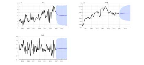
Fig. 1. Forecasts for Australia tourist visits (AU), Australian dollar— Indonesian rupiah exchange rate (AUD) and inflation for 2017—2018 (INFL).
As can be seen from Fig. 1 the number of visits decrease during 2017 and roughly equal 80,000 visits for 2018 (see the blue line under the title AU). The Australian dollar to Indonesian Rupiah exchange rates shows a slightly increasing trend, but the values close to 10,500. Inflation is relatively stable and reached 0.2 level.
and for Σ ~ IW (S0 ,α0) which has the form
Oo+n+1
f (∑)α l∑l 2 exp
Refer to in [6] or [7] for further discussion of the above priors.
C. Posterior Distribution
Posterior for normal-Wishart prior has the following closed form
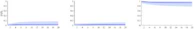
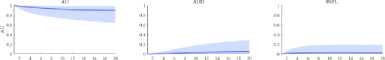
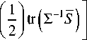
Fig. 2. Forecast error decomposition.
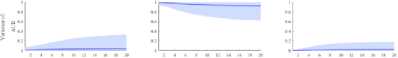
The dynamical relationship between endogenous variables can be seen in Fig. 3. It can be seen clearly that there are shocks at the beginning period for all variables.
α+n+1
×∣∑∣ 2 exp
Inference for posterior distribution can be obtained by using Markov Chain Monte Carlo and since the posterior has closed form Gibbs sampling can be used, see for instance [8] or [9].
III. RESULTS
In this research, we obtained the Australian tourist visits from the Bali Tourism Department. The data is available from January 2010 to September 2017. However, we use the data up to December 2016 and use the remaining data to compare forecast and actual data. The exchange rate data was obtained from Bank Indonesia (Indonesian Reserve Bank) and the monthly inflation rates were obtained from the website www.investing.com. Note that inflation rates in Australia are published quarterly. Thus, the monthly inflation rates used here is Melbourne's Institute inflation
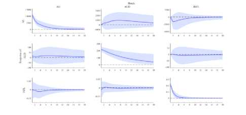
Fig. 3. Forecasts for Australia tourist visits (AU), Australian dollar— Indonesian rupiah exchange rate (AUD) and inflation for 2017—2018 (INFL).
Fig.4 describes the structural shocks for all three variables.
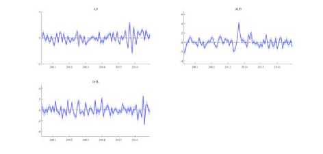
Fig. 3. Structural shocks for the three variables: AU, AUD, and INFL.
Analysis,”Studies in Nonlinear Dynamics and Econometrics, vol. 9, pp. 1-34, 2005.R. J. Vidmar.(1992, August).On the use of atmospheric plasmas as electromagnetic reflectors.IEEE Trans. Plasma Sci. [Online].21(3). Pp. 876–880.
-
IV. CONCLUSION
Forecasts for three variables suggest that the tourist visits decrease and for inflation stabilized at 2% level and exchange rate close to 10,500. Impulse response functions for all variables clearly show some shocks in the early period before reaching zero.
Acknowledgment
We would like to thank the Faculty of Mathematics and Natural Sciences for the research grant under the scheme Hibah Unggulan Program Studi contract number 3634/UN14.2.8.II/LT/2017 dated 5 July 2017.
References
-
[1] V. Cho, “Tourism forecasting and its relationship with leading economic indicators,” Journal of Hospitality and Tourism Research, vol. 25, pp. 399-420, 2001.
-
[2] M. Lu, “Vector Autoregression (VAR) - An Approach to Dynamic Analysis of Geographic Processes,” Geografiska Annaler. Series B, Human Geography, vol. 83, pp. 67-78, 2001.
-
[3] H. Lütkepohl and M. Kratzig, Eds., Applied Time Series Econometrics. Cambridge: Cambridge University Press, 2004.
-
[4] H. Lütkepohl, New Introduction to Multiple Time Series Analysis. Berlin: Springer, 2005.
-
[5] R. S. Tsay, Multivariate Time Series Analysis with R and Financial Applications. New Jersey: Wiley, 2014.
-
[6] G. Koop and D. Korobilis, “Bayesian Multivariate
Time Series Methods for Empirical
Macroeconomics,”Foundations and Trends in Econometrics, vol. 3, pp. 267-358, 2010.
-
[7] S. Karlsson, “Forecasting with Bayesian Vector Autoregression,” in Handbook of Economic Forecasting. Vol. Volume 2, Part B, E. Graham and T. Allan, Eds., ed: Elsevier, 2013, pp. 791-897.
-
[8] S. Karlsson, “Forecasting with Bayesian Vector Autoregression,” in Handbook of Economic Forecasting, ed: Elsevier, 2013.
-
[9] A. Dieppe, R. Legrand, and B. v. Roye, “The BEAR toolbox,” in Working Paper Series ed.
https://www.ecb.europa.eu/pub/pdf/scpwps/ecbwp1934 .en.pdf: European Central Bank (ECB), 2016.
-
[10] V. Ivanov and L. Kilian, “A Practitioner’s Guide to Lag Order Selection for VAR Impulse Response
Discussion and feedback