MODIFIED ARMIJO RULE ON GRADIENT DESCENT AND CONJUGATE GRADIENT
on
E-Jurnal Matematika Vol. 6 (3), Agustus 2017, pp. 196-204
DOI: https://doi.org/10.24843/MTK.2017.v06.i03.p166
ISSN: 2303-1751
MODIFIED ARMIJO RULE ON GRADIENT DESCENT AND CONJUGATE GRADIENT
Zuraidah Fitriah1§, Syaiful Anam2
1Mathematics Department Brawijaya University [Email: zuraidahfitriah@ub.ac.id] 2Mathematics Department Brawijaya University [Email: syaiful@ub.ac.id] §Corresponding Author
ABSTRACT
Armijo rule is an inexact line search method to determine step size ak in some descent method to solve unconstrained local optimization. Modified Armijo was introduced to increase the numerical performance of several descent algorithms that applying this method. The basic difference of Armijo and its modified are in existence of parameter μ ∈ [0,2) and estimating parameter Lk that be updated in every iteration. This article is comparing numerical solution and time of computation of gradient descent and conjugate gradient hybrid Gilbert-Nocedal (CGHGN) that applying modified Armijo rule. From program implementation in Matlab 6, its known that gradient descent was applying modified Armijo more effectively than CGHGN from one side: iteration needed to reach some norm of gradient Hgk ∣∣ (input by the user). The amount of iteration was representing how long the step size of each algorithm in each iteration. In another side, time of computation has the same conclusion.
Keywords: Armijo line search; conjugate gradient hybrid Gilbert-Nocedal; gradient descent; modified Armijo line search
Optimization is still an interesting issue to be learned and developed, especially numerical methods for finding solutions. This is known as numerical optimization. Optimization is the process of finding the optimal solution of a problem either with constraints or without constraints. Numerical optimization allows the discovery of solutions to problems that are difficult to be solved analytically.
The optimization problem is essentially a matter of minimizing a function f(x). As for maximization, a function f(x) can also be formed as a minimization problem of function -f(x). To solve the minimization problem, some descent iterative methods have been introduced, including gradient descent (steepest descent) and conjugate gradient methods. These two methods are just some of the many methods that can be used to solve local optimization problems. There is much useful application of gradient descent method. One of them is to find the saddle point of a complex integral (Wang, 2008). While Chen (2009) use gradient descent to fit the measured data of laser
grain-size distribution of the sediments.
While in the conjugate gradient method itself there are various types of parameter determination βk. In this paper, we will use conjugate gradient hybrid Gilbert-Nocedal which is a hybrid of Fletcher-Reeves conjugate gradient (FR) and Polak-Ribiere-Polyak conjugate gradient (PRP).
Gradient descent and conjugate gradient algorithms start with determining the initial point to run the first iteration. The next points will be obtained from each iteration in which the conditions determined will converge to the optimum solution of the optimization objective function. One important part of these two algorithms is the determination of step size (ak) on each iteration. This step size determination can be done in many ways called line search. One of the line search rules often used is Armijo rule.
To improve the numerical performance of Armijo rules, Shi (2005) have introduced and developed Armijo modification rules. The difference with classical Armijo is the value of parameter μ ∈ [0,2) and Lk which is updated on each iteration with a certain estimate. In modified
Armijo rules, it is easier to obtain larger step sizes, meaning that with the same stopping criteria, the iterations required by a descent algorithm will be less than using classical Armijo. This will be compared to the gradient descent and conjugate gradient hybrid Gilbert-Nocedal algorithms. Likewise, the time required for each algorithm to solve the optimization problem by applying the classical Armijo rules and its modification in step size determination.
Gradient descent is one of the optimization algorithms for the problem of unconstrained minimization. The problem is to minimize f :I → W,I ⊂ Wn. The iteration renews xk so that in the end of iterations, there is an approximation of the above minimization problem. To find the local minimum of a function using gradient descent, one of the important steps is to determine the descent direction, dk, as the negative of the gradient gk = Vf(x) of the objective function f (x) at ktfl iteration point. Next, select the step size ak by using line search, either in exact or inexact.
For more details about this method, the following is gradient descent algorithm.
Step 0. Given starting point x0, k — 0.
Step 1. Select the descent direction d k — -gk. If d k — 0, then the iteration stops.
Step 2. Select step size ak using line search method (either exact or not exact).
Step 3. Renew the point xk+1 — xk + akdk,k — k + 1. Return to step 1.
The iteration stops if the iteration termination criterion has been reached. for example if the k -th point is close enough to the minimum point of the destination function.
Suppose that a quadratic function optimization problem will be solved as follows.
1
M in f (x) — χxτ X x + Qτx
The descent direction, dk, of the conjugate gradient is Qconjugate vectors, where Q is the positive definite matrix found in the function f(x) above.
Suppose given a starting point . The descent direction for the starting point uses the descent direction of the descent gradient algorithm i.e
do — -9o — -^f(χo).
In this paper, the descent direction, dk, is determined as follows:
H = [-®k, k — 0
-
k -~∂k + kk^-k- 1, k ≥ 1
Where gk — Vf (xk) and βk are parameters. Actually, there are several types of conjugate gradient algorithm based on an estimation of parameter βk. Some of them by Andrei (2007) are as follows:
-
• Fletcher-Reeves (FR) conjugate gradient βPR _ __ggkggk__
-
gk-1gk
-
• Poly-Ribiere-Polyak (PRP) conjugate gradient
rPRP _ gIcVk
P k τ ,Vk gk gk-1
gk-1gk-1
-
• Dai-Yuan (DY) conjugate gradient
T ody _gkgk P k —~ ,yk—gk-gk-1,
yk⅛
sk — xk- x--l
-
• Hestenes-Stiefel (HS) conjugate gradient ons gkVk _
β k τ ,Vk gk gk-1,
yk¾
sk — xk- xk-l
-
• Conjugate descent (CD)
T n CD gkgk
β k —-~---~>sk~xk~x1-g
gk-1^k
-
• Liu-Storey (LS) conjugate gradient
ols _ glyk
βk — -~ ~'sk~xk~x1-g
gk-1^k
In addition to several types of determination of the parameters of βk mentioned above, there are also some hybrids of the types that have been developed. But in this paper will be used conjugate gradient hybrid Gilbert-Nocedal as follows.
-
-βkR if βPRP < f-.
-
βkn{∖ β^rp if Wrp∖≤ββκ, Ir if βRRP > βRp.
It can be written briefly,
βRN — max{-βRR,min{βRRP,βRR)}.
For more details about this method, here is the conjugate gradient algorithm.
Step 0. Given starting point x0, k0.
Step 1. For k — 0,dk — -gk. For k ≥ 1, find βk, dk — -gk + βkdk-1. If dk — 0, then the iteration stops.
Step 2. Select step size ak using line search method (either exact or not exact).
Step 3. Renew the point xk+1 — xk + akdk,k —
k + 1. Return to step 1.
To determine the step size, ak, there are many line search methods that can be used, either in exact or inexact. One method of line search that is not exact is the rule of Armijo.
The Armijo rules in determining step size are as follows:
ak = max{Sk,βsk, β2sk,...}
That fulfills
f fa + adk) -fk≤ aagldk
Where
sk — -ιg∏v,β ∈ (0,1),α ∈ (0,1),l > 0 L∣∣dk∣r ∖ 2/
In this modified Armijo rule, it will be found that the step size, ak, which is defined as greater than that defined in the classic Armijo rules. In other words, the step size defined on the modified Armijo rule is easier to find than the step size in the classic Armijo rules.
The modified Armijo Rules by Shi (2005) are as follows:
Determine the scalars sk, β, Lk, μ, and α, where gldk
sk — LkWdkW2'
β ∈ (0,1), Lk >0,μ∈[0,2), a ∈(θ,-), and ak is the largest a scalar in {sk, βsk, β2sk,...,} such that
f(xk + adk}-fk ≤ aa [gkdk + 1aμLk∖∖dk∖∖2]
In the modified Armijo rule there is a parameter that needs to be estimated and updated on each iteration, ie Lk. Here is the difference between the classic Armijo rules and it's modified, as well as the μ parameter. In the classic Armijo rule, the parameter L is not updated on each iteration. Lk in the modified Armijo rule can be approximated by the Lipschitz constant of the gradient g(x) of the objective function f(x), M'. If M' is given, then, of course, can be taken Lk = M'. However, M' is often unknown in many cases, so the Lk parameter can be estimated in one of the following ways.
Let δk-1 — xk- xk-1, Vk-I = gk- gk-1, k = 2,3,4,... Then the parameter value Lk can be determined as follows.
Lk —
Wyk-ιW
Wδk-1W
or
Lk —max{w⅛ =1,2.....m}
Where k ≥ M + 1, M is a positive integer. The second way to estimate these parameters is as
follows.
or
Lt=⅛-y-
Lk — max
^ t∣l<⅛-ill2
1 k-iyk-i .
i — 1,2.....M
The third way is as follows.
j _ Wyk-1W2
Lk or
⅛-1yk-ι
or
}
l (WVk-iW2
Lk — max i —1,2,.,M f
δk-iVk-i
As for k — 1 taken L1 — 1.
The above estimates are just a few of the many ways to estimate M'. The above estimates will be used in the gradient descent and conjugate gradient hybrid Gilbert-Nocedal (CGHGN) algorithms which contain modifications to Armijo's rules in it (Shi, 2005).
The gradient descent algorithm with modified Armijo rules, as described in the above sections, is applied to Matlab 6 software, with an estimated parameter Lk, various scalar inputs β,α,μ maximum iteration, and maximum errors ε.
The numerical results of two variable test functions using gradient descent algorithm with estimated parameter Lk — W^J^1^’ the parameter value is selected β — 0.87, a — 0.38, Maximum iteration 100, and the maximum difference between analytical solutions and numerical solutions ε = 0.005, listed in Table 1 below. Iteration will stop if either one of the maximum iterations or the maximum difference between the analytical solution and the numerical solution is reached. In each of the following tables, compare the numerical solution of the test function with the parameter value range μ at [0,2).
From Table 1 below it can be seen that in a simple function, with μ> 0, there are fewer
iterations and ∣∣μkH is much smaller. μ = 0 represents the classical Armijo rule with L = 1, not updated on each iteration, whereas μ> 0 represents the modified Armijo rule with Lk updated on each iteration. While on the Quadric function, the gradient descent with modified Armijo works better than the classic Armijo. This is demonstrated by the achievement of∣μkH which is not much different, modified Armijo requires much less iteration. In the Zakharof function, of the number of iterations, the classical Armijo seems to work a little better than the modification. However, the ∣∣μkH obtained by Armijo modification is slightly smaller than the classic Armijo. Almost the same in Himmenblau function, on some values μ, modified Armijo works a little better, but on some other μ values, on the contrary, it works a little worse than the classic Armijo.
Table 1. Numerical Results of Two Variable Test Functions with Gradient Descent
|
μ |
Number of iteration (⅛) |
E |
M |
|
Quadric function with x0 |
(1,2) | ||
|
0 |
20 |
5.961 (10-6) |
0.0043994 |
|
0.5 |
4 |
2.3624 (10-6) |
0.0045728 |
|
1.0 |
4 |
1.2997 (10-5) |
0.0048104 |
|
1.5 |
4 |
1.2997 (10-5) |
0.0048104 |
|
1.99 |
4 |
1.2997 (10-5) |
0.0048104 |
|
Zakharof function with x 0 (1,2) | |||
|
0 |
4 |
7.381 (10-8) |
0.00081505 |
|
0.5 |
6 |
5.181(10-9) |
0.00021548 |
|
1.0 |
6 |
5.181(10-9) |
0.00021548 |
|
1.5 |
6 |
5.181(10-9) |
0.00021548 |
|
1.99 |
6 |
5.181(10-9) |
0.00021548 |
|
De Jong function with x 0 |
(1,2) | ||
|
0 |
4 |
1.0207 (10-6) |
0.0020206 |
|
0.5 |
2 |
9.9104 (10-29) |
1.991 (10-14) |
|
1.0 |
2 |
2.4155 (10-28) |
3.1048 (10-14) |
|
1.5 |
2 |
2.4155 (10-28) |
3.1048 (10-14) |
|
1.99 |
2 |
2.4755 (10-28) |
3.1468 (10-14) |
|
Himmenblau function with x 0 (0,0) | |||
|
0 |
14 |
1.9501 (10-7) |
0.0033515 |
|
0.5 |
12 |
2.0832 (10-8) |
0.0015424 |
|
1.0 |
12 |
1.6794 (10-7) |
0.0032052 |
|
1.5 |
10 |
3.8923 (10-8) |
0.0014833 |
|
1.99 |
17 |
2.5695 (10-7) |
0.0039309 |
|
McCormic function with x |
0 (0,0) | ||
|
0 |
8 |
1.9132 |
0.0020333 |
|
0.5 |
7 |
1.9132 |
0.0020157 |
|
1.0 |
7 |
1.9132 |
0.0023628 |
|
1.5 |
5 |
1.9132 |
0.0048835 |
|
1.99 |
5 |
1.9132 |
0.0016221 |
With a bit more iteration but ∣∣μkH which is also slightly smaller, in Zakharof and Himmenblau functions, it cannot be concluded that gradient descent with Armijo modification is not better than gradient descent with classic Armijo, although it cannot be concluded otherwise. Moreover, it turns out the numerical results of the De Jong function show again that modified Armijo is still better than classic Armijo.
Figures 1.a and 1.b below show the different results of the gradient descent iteration using classic Armijo with those using modified Armijo. From the figure, it can be seen that the modified Armijo requires fewer iterations to satisfy the termination criteria ( ε < 0.005). In other words, modified Armijo converges faster on the minimum solution of the optimization problem.
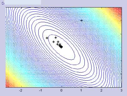
Figure 1.a Gradient Descent with Classic Armijo (μ = 0) on Quadric Function
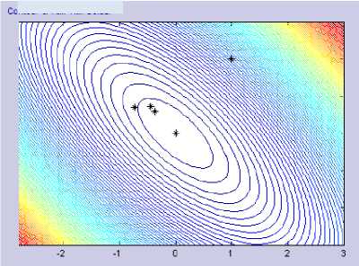
Figure 1.b Gradient Descent with Modified Armijo on Quadric Function
While Figure 2.a and 2.b show differences in the effect of parameter values μ. With larger μ, the step size will be larger.
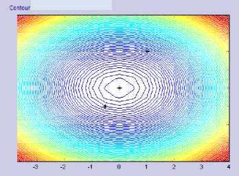
Figure 2.a Gradient Descent with Modified Armijo on
DeJong Function (μ = 1,μ = 1.5)
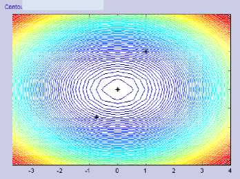
Figure 2.b Gradient Descent with Modified Armijo on
DeJong Function (μ = 1.99)
To summarize in general this comparison, then there should be test functions with larger dimensions to test the method. The parameters used are the same as the parameters used in the two-dimensional test function in Table 1. But the termination criterion used is different, ie if it has reached maximum iteration 1000 iterations or IIgfcH < 0.005. The numerical results of gradient descent with classical Armijo rules and its modified on large-dimensional test functions are presented in Table 2 and Table 3.
Using a four-dimensional test function, it can be seen that gradient descent with modified Armijo works better in terms of a number of iterations required to achieve the same HgfcH than the classical Armijo that is < 0.005. In each of the four-dimensional functions in Table 2, modified Armijo always works better than the classical Armijo, even though the termination requirement (ε < 0.005) is same, the modified Armijo still gets a smaller HgfcH than the classic Armijo, with much less number of iterations. In Powell Singular function, if the iteration is not limited to 1000 iterations, then to get the expected HgfcH, the process has not been completed. That means the required iteration will be much more than the modified Armijo. In Powell Singular, Watson, Trigonometric, and Penalty II functions, it is also generated that the iterations needed will be less as
the parameter value of μ is greater. This proves that selection of this parameter value has important value in modified Armijo.
Similarly, for the 8 dimension test function, the results can be seen in Table 3. At Watson function, it is seen that there is a significant decrease in the number of iterations of the classical Armijo application to the application of its modification. While in Penalty II, there was also a decrease in the number of iterations although not as significant in the Watson function. This further reinforces the assumption of early test functions that modified Armijo works better than classical Armijo on the gradient descent algorithm.
Table 2. The Numerical Result of 4 Dimension Test Function with Gradient Descent
|
μ |
Number of iteration(fc) |
E |
HgfcH |
|
4 dimension Powell Singular function with x 0 (1,1,1,1) | |||
|
0 |
1000 |
0.00040193 |
0.013225 |
|
0.5 |
279 |
0.00020607 |
0.0049055 |
|
1.0 |
209 |
0.00020451 |
0.0049746 |
|
1.5 |
182 |
0.00020795 |
0.0049696 |
|
1.99 |
169 |
0.00020783 |
0.0049937 |
|
4 dimension Watson function with x0 (0,0,0,0) | |||
|
0 |
410 |
0.0060494 |
0.0047514 |
|
0.5 |
129 |
0.0060433 |
0.0042924 |
|
1.0 |
100 |
0.0060441 |
0.0044026 |
|
1.5 |
96 |
0.0060496 |
0.0047381 |
|
1.99 |
83 |
0.0060247 |
0.0039382 |
|
4 dimension Penalty function with x0 (1,2,3,4) | |||
|
0 |
84 |
0.0062071 |
0.004998 |
|
0.5 |
2 |
0.0017474 |
0.001944 |
|
1.0 |
2 |
0.0017474 |
0.001944 |
|
1.5 |
2 |
0.0017474 |
0.001944 |
|
1.99 |
2 |
0.0017474 |
0.001944 |
|
4 dimension Variably-Dimensioned function with x0 (0,0,0,0) | |||
|
0 |
98 |
2.6045 (10-6) |
0.0049899 |
|
0.5 |
17 |
1.2441 (10-9) |
0.00039367 |
|
1.0 |
17 |
1.2441 (10-9) |
0.00039367 |
|
1.5 |
17 |
1.2441 (10-9) |
0.00039367 |
|
1.99 |
17 |
1.2441 (10-9) |
0.00039367 |
|
4 dimension Trigonometric function with x0 (0.25,0.25,0.25,0.25) | |||
|
0 |
18 |
0.00035521 |
0.0039039 |
|
0.5 |
12 |
0.00033347 |
0.0036763 |
|
1.0 |
10 |
0.00040127 |
0.0046417 |
|
1.5 |
10 |
0.00039599 |
0.004532 |
|
1.99 |
10 |
0.00038882 |
0.0044509 |
|
4 dimension Penalty II function with x 0 (1,1,1,1) | |||
|
0 |
16 |
0.82485 |
0.0046897 |
|
0.5 |
13 |
0.82485 |
0.0035263 |
|
1.0 |
12 |
0.82485 |
0.002263 |
|
1.5 |
12 |
0.82485 |
0.002263 |
|
1.99 |
12 |
0.82485 |
0.002263 |
Table 3. The Numerical Result of 8 Dimension Test Function with Gradient Descent
|
μ |
Number of iteration (k) |
E |
HgfcH |
|
8 dimension Watson function with x0 (0,0,0,0,0,0,0,0), maximum number of iterations:1000, ε < 0.05 | |||
|
0 |
249 |
0.0056431 |
0.049389 |
|
0.5 |
87 |
0.0060244 |
0.049453 |
|
1.0 |
55 |
0.0060305 |
0.048821 |
|
1.5 |
56 |
0.005936 |
0.047586 |
|
1.99 |
48 |
0.0061168 |
0.048974 |
|
8 dimension Penalty II function with x0 (1,1,1,1,2,2,2,2), maximum number of iterations:1000, ε < 0.005 | |||
|
0 |
16 |
0.82494 |
0.0046897 |
|
0.5 |
13 |
0.82494 |
0.0035121 |
|
1.0 |
12 |
0.82494 |
0.0021299 |
|
1.5 |
12 |
0.82494 |
0.0021299 |
|
1.99 |
12 |
0.82494 |
0.0021299 |
After comparing classical Armijo and its modification to the gradient descent algorithm, here is the next comparison on CGHGN. The test functions used remain the same as the test functions in the above sections. Similarly, for the value of the parameters used and the iteration termination criterion.
From Table 4 it is generally found that conjugate gradient does not work better than gradient descent in applying modified Armijo. This can be seen from the numerical results on Quadric, Himmenblau, and Zakharof functions. Even the performance is very bad on the Quadric function, with more iterations needed to achieve the same HgfcII stopping criteria. Also, the HgfcH obtained is worse than the classic Armijo.
Table 4. The Numerical Results of The Two
Variable Test Function with CGHGN
|
μ |
Number of iteration (k) |
E |
HgfcH |
|
Quadric function with x 0 : |
(1,2) | ||
|
0 |
8 |
9.435 (10-7) |
0.0020482 |
|
0.5 |
18 |
3.7116 (10-6) |
0.0028629 |
|
1.0 |
15 |
1.0485 (10-5) |
0.0041436 |
|
1.5 |
19 |
4.9341 (10-6) |
0.003629 |
|
1.99 |
13 |
7.0949 (10-6) |
0.0033074 |
|
Zakharof function with x0 |
: (1,2) | ||
|
0 |
4 |
7.3802 (10-8) |
0.00081502 |
|
0.5 |
6 |
5.1685 (10-9) |
0.00021537 |
|
1.0 |
6 |
5.1685 (10-9) |
0.00021537 |
|
1.5 |
6 |
5.1685 (10-9) |
0.00021537 |
|
1.99 |
6 |
5.1685 (10-9) |
0.00021537 |
|
De Jong function with x 0 : |
(1,2) | ||
|
0 |
4 |
1.0207 (10-6) |
0.0020206 |
|
0.5 |
2 |
1.7711 (10-28) |
2.6617 (10-14) |
|
1.0 |
2 |
6.7025 (10-28) |
5.1778 (10-14) |
|
1.5 |
2 |
6.7025 (10-28) |
5.1778 (10-14) |
|
1.99 |
2 |
1.6852 (10-27) |
8.2102 (10-14) |
|
Himmenblau function with x 0 (0,0) | |||
|
0 |
12 |
8.8547 (10-8) |
0.0039747 |
|
0.5 |
13 |
4.732 (10-8) |
0.0018234 |
|
1.0 |
23 |
4.1353 (10-7) |
0.0046038 |
|
1.5 |
15 |
3.2192 (10-8) |
0.0033049 |
|
1.99 |
12 |
2.4744 (10-7) |
0.0033668 |
|
McCormic function with x 0 (0,0) | |||
|
0 |
6 |
1.9132 |
0.0038449 |
|
0.5 |
7 |
1.9132 |
0.0045575 |
|
1.0 |
8 |
1.9132 |
0.0026397 |
|
1.5 |
7 |
1.9132 |
0.0016163 |
|
1.99 |
10 |
1.9132 |
0.0041537 |
The CGHGN iteration behavior using both classical Armijo and its modification is not so different. It can be seen in Figure 4.a-d below. With various parameter values μ, the resulting iteration points are not much different in Himmenblau function.
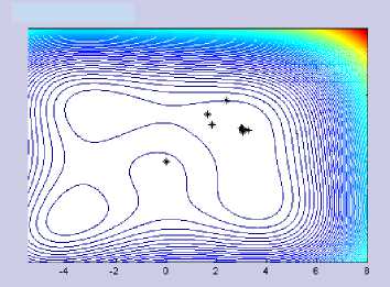
Figure 4.a CGHGN with Classic Armijo (μ = 0) on Himmenblau Function
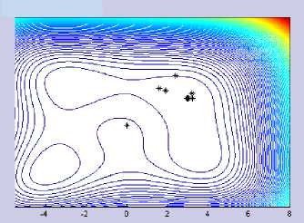
Figure 4.b CGHGN with Modified Armijo (μ = 0.5) in Himmenblau Function
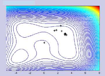
Figure 4.c CGHGN with Modified Armijo (μ = 1) in Himmenblau Function
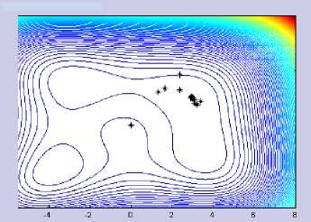
Figure 4.d CGHGN with Modified Armijo (μ = 1.5) in Himmenblau Function
Table 5 below shows CGHGN numerical results with modified Armijo on four-dimensional functions. The result is that CGHGN works very badly in applying modified Armijo.
Tabel 5. Numerical Result 4-dimensional Test Function with CGHGN
|
μ |
Number of iteration (k') |
E |
llf⅛ll |
|
4-dimensional Powell Singular function with x 0 (1,1,1,1) | |||
|
0 |
74 |
2.5467 (10-5) |
0.0033689 |
|
0.5 |
1000 |
0.00053896 |
0.016547 |
|
1.0 |
1000 |
0.00052487 |
0.016728 |
|
1.5 |
1000 |
0.00052992 |
0.015748 |
|
1.99 |
1000 |
0.00053591 |
0.016243 |
|
4-dimensional Watson function with x0 (0,0,0,0) | |||
|
0 |
34 |
0.0060263 |
0.003837 |
|
0.5 |
462 |
0.0060228 |
0.0041832 |
|
1.0 |
528 |
0.0060492 |
0.004726 |
|
1.5 |
449 |
0.0060409 |
0.003878 |
|
1.99 |
559 |
0.0060495 |
0.0048206 |
|
4-dimensional Penalty function with x0 (1,2,3,4) | |||
|
0 |
84 |
0.0062071 |
0.004998 |
|
0.5 |
2 |
0.0017474 |
0.001944 |
|
1.0 |
2 |
0.0017474 |
0.001944 |
|
1.5 |
2 |
0.0017474 |
0.001944 |
|
1.99 |
2 |
0.0017474 |
0.001944 |
|
4-dimensional Variably-Dimensioned with x0 (0,0,0,0) | |||
|
0 |
12 |
8.7638 (10-7) |
0.0018735 |
|
0.5 |
85 |
2.3254 (10-6) |
0.0041347 |
|
1.0 |
77 |
3.2597 (10-6) |
0.0047175 |
|
1.5 |
46 |
5.3615 (10-6) |
0.0047064 |
|
1.99 |
76 |
4.195 (10-6) |
0.0048226 |
|
4-dimensional Trigonometric funtion with x0 (0.25,0.25,0.25,0.25) | |||
|
0 |
12 |
0.00040346 |
0.0049897 |
|
0.5 |
23 |
0.00034834 |
0.0034499 |
|
1.0 |
20 |
0.00037274 |
0.0044723 |
|
1.5 |
23 |
0.00034909 |
0.0038791 |
|
1.99 |
20 |
0.00037369 |
0.0049191 |
|
4-dimensional Penalty II function with x 0 (1,1,1,1) | |||
|
0 |
11 |
0.82484 |
0.00081602 |
|
0.5 |
18 |
0.82484 |
0.00092696 |
|
1.0 |
18 |
0.82485 |
0.0042525 |
|
1.5 |
20 |
0.82485 |
0.0033585 |
|
1.99 |
21 |
0.82485 |
0.003335 |
In Table 5, it can be seen that the conjugate gradient only works well on the Penalty function. While in other functions, to meet the same termination criteria (ε < 0.005), conjugate gradient with modified Armijo requires much more iteration. This is enough to show the ineffectiveness of Armijo modification if applied to this algorithm. In contrast, in Table 1 and Table 2, CGHGN with Classical Armijo works better than if classical Armijo is applied to the gradient descent. However, as discussed in this paper is how effective modified Armijo is applied to the
gradient descent and CGHGN, it is sufficient to answer that modified Armijo works more effectively on the gradient descent.
In addition to comparing numerical solutions of each algorithm by applying classical Armijo and its modifications, it can be compared computation time, ie the time required by the algorithm to solve the problem of minimizing the test functions until the desired stopping criterion is reached. Before reading the tables below, by comparison of the number of iterations as described in the above sections, it is possible to guess the computational time behavior required for each algorithm. For gradient descent, the average number of iterations decreases, so too is the computation time.
Tabel 6. Computational Time of Gradient Descent and CGHGN on Two-dimensional Function
|
μ |
Gradient Descent |
CGHGN | ||
|
E |
t |
E |
t | |
|
Zakharof function | ||||
|
0 |
7.381 (10-8) |
0.016 |
7.3802 (10-8) |
0.016 |
|
0.5 |
5.181(10-9) |
0.016 |
5.1685 (10-9) |
0.015 |
|
1.0 |
5.181(10-9) |
0.016 |
5.1685 (10-9) |
0.016 |
|
1.5 |
5.181(10-9) |
0.016 |
5.1685 (10-9) |
0.015 |
|
1.99 |
5.181(10-9) |
0 |
5.1685 (10-9) |
0.016 |
|
De Jong function | ||||
|
0 |
1.0207 (10-6) |
0 |
1.0207 (10-6) |
0.015 |
|
0.5 |
9.9104 (10-29) |
0.016 |
1.7711 (10-28) |
0.016 |
|
1.0 |
2.4155 (10-28) |
0 |
6.7025 (10-28) |
0.016 |
|
1.5 |
2.4155 (10-28) |
0 |
6.7025 (10-28) |
0.015 |
|
1.99 |
2.4755 (10-28) |
0 |
1.6852 (10-27) |
0.016 |
|
Himmenblau function | ||||
|
0 |
1.9501 (10-7) |
0.031 |
8.8547 (10-8) |
0.031 |
|
0.5 |
2.0832 (10-8) |
0.015 |
4.732 (10-8) |
0.016 |
|
1.0 |
1.6794 (10-7) |
0.015 |
4.1353 (10-7) |
0.016 |
|
1.5 |
3.8923 (10-8) |
0.016 |
3.2192 (10-8) |
0.016 |
|
1.99 |
2.5695 (10-7) |
0.016 |
2.4744 (10-7) |
0 |
|
McCormic function | ||||
|
0 |
1.9132 |
0.875 |
1.9132 |
0.016 |
|
0.5 |
1.9132 |
0.406 |
1.9132 |
0.015 |
|
1.0 |
1.9132 |
0.016 |
1.9132 |
0.016 |
|
1.5 |
1.9132 |
0.015 |
1.9132 |
0.016 |
|
1.99 |
1.9132 |
0.015 |
1.9132 |
0.016 |
In Table 6 have not been able to prove the guess because the computation time difference is not so large on each parameter value μ, both on the gradient descent and on CGHGN. However, in Table 7, and Table 8 with larger dimensioned functions, it can prove that guess because the
computation time difference is large enough for each parameter change, especially from the value of μ = 0 to other μ values. The considerable computation time difference can be seen, among others, on 4-dimension Powell Singular function and 4-dimension and 8-dimension Watson function. Gradient descent shows better results than CGHGN in terms of computational time in applying modified Armijo on average test function used, either 2, 4, or, 8-dimension.
Tabel 7. Computational Time of Gradient Descent and CGHGN on Four-dimensional Function
|
μ |
Gradient Descent |
CGHGN | ||
|
E |
t |
E |
t | |
|
4 dimension Powell Singular function | ||||
|
0 |
0.00040193 |
2.156 |
2.5467 (10-5) |
0.078 |
|
0.5 |
0.00020607 |
0.125 |
0.00053896 |
1.031 |
|
1.0 |
0.00020451 |
0.094 |
0.00052487 |
1.015 |
|
1.5 |
0.00020795 |
0.078 |
0.00052992 |
0.985 |
|
1.99 |
0.00020783 |
0.062 |
0.00053591 |
0.985 |
|
4 dimension Watson function | ||||
|
0 |
0.0060494 |
10.11 |
0.0060263 |
0.578 |
|
0.5 |
0.0060433 |
0.75 |
0.0060228 |
3.969 |
|
1.0 |
0.0060441 |
0.578 |
0.0060492 |
4.391 |
|
1.5 |
0.0060496 |
0.547 |
0.0060409 |
3.734 |
|
1.99 |
0.0060247 |
0.438 |
0.0060495 |
4.219 |
|
4 dimension Penalty function | ||||
|
0 |
0.0062071 |
0.031 |
0.0062071 |
0.032 |
|
0.5 |
0.0017474 |
0.016 |
0.0017474 |
0.016 |
|
1.0 |
0.0017474 |
0.016 |
0.0017474 |
0.015 |
|
1.5 |
0.0017474 |
0.015 |
0.0017474 |
0.015 |
|
1.99 |
0.0017474 |
0.016 |
0.0017474 |
0.015 |
|
4 dimension Variably-Dimensioned function | ||||
|
0 |
2.6045 (10-6) |
0.266 |
8.7638 (10-7) |
0.062 |
|
0.5 |
1.2441 (10-9) |
0.016 |
2.3254 (10-6) |
0.078 |
|
1.0 |
1.2441 (10-9) |
0.016 |
3.2597 (10-6) |
0.063 |
|
1.5 |
1.2441 (10-9) |
0.015 |
5.3615 (10-6) |
0.047 |
|
1.99 |
1.2441 (10-9) |
0.015 |
4.195 (10-6) |
0.062 |
|
4 dimension Trigonometric function | ||||
|
0 |
0.00035521 |
0.031 |
0.00040346 |
0.015 |
|
0.5 |
0.00033347 |
0.015 |
0.00034834 |
0.031 |
|
1.0 |
0.00040127 |
0.015 |
0.00037274 |
0.032 |
|
1.5 |
0.00039599 |
0.015 |
0.00034909 |
0.031 |
|
1.99 |
0.00038882 |
0.015 |
0.00037369 |
0.032 |
|
4 dimension Penalty II function | ||||
|
0 |
0.82485 |
0.125 |
0.82484 |
0.094 |
|
0.5 |
0.82485 |
0.031 |
0.82484 |
0.032 |
|
1.0 |
0.82485 |
0.016 |
0.82485 |
0.031 |
|
1.5 |
0.82485 |
0.015 |
0.82485 |
0.047 |
|
1.99 |
0.82485 |
0.015 |
0.82485 |
0.032 |
Table 8. Computational Time of Gradient Descent and CGHGN on Eight-dimensional Function
|
μ |
Gradient Descent |
CGHGN | ||
|
E |
t |
E |
t | |
|
Fungsi Watson dimensi 8 | ||||
|
0 |
0.0056431 |
40.39 |
0.0039089 |
3.5 |
|
0.5 |
0.0060244 |
3.703 |
0.0056966 |
14.266 |
|
1.0 |
0.0060305 |
2.25 |
0.0056511 |
16.031 |
|
1.5 |
0.005936 |
2.25 |
0.0054967 |
15.954 |
|
1.99 |
0.0061168 |
2.047 |
0.0053083 |
17.266 |
|
Fungsi Penalty II dimensi 8 | ||||
|
0 |
0.82494 |
0.125 |
0.82494 |
0.078 |
|
0.5 |
0.82494 |
0.047 |
0.82494 |
0.046 |
|
1.0 |
0.82494 |
0.047 |
0.82494 |
0.062 |
|
1.5 |
0.82494 |
0.031 |
0.82494 |
0.063 |
|
1.99 |
0.82494 |
0.031 |
0.82494 |
0.078 |
Of the two comparable parameters, a number of iterations required to achieve a required stopping criterion and computational time required to solve numerical minimization problem, it has been shown that gradient descent is better and more effective than CGHGN in applying the modified Armijo rule.
REFERENCES
-
H. Chen. 2009. Application of Gradient Descent Method to The Sedimentary Grain-Size Distribution Fitting. Journal of Computational and Applied Mathematics, vol.233, pp. 11281138.
-
N. Andrei. 2007. New Hybrid Conjugate Gradient Algorithm as A Convex Combination of PRP and DY for Unconstrained Optimization. Journal of Research Institute for Informatics.
-
X. Wang. 2008. Method of Steepest Descent and Its Application. University of Tennessee, Knoxville.
Z.J. Shi and J. Shen. 2005. New Inexact Line Search Method for Unconstrained Optimization. Journal of Optimization Theory and Applications, Vol.127 No.2, pp. 425-446.
4. CONCLUSIONS
From the discussion above, it can be concluded that modified Armijo works very well on the gradient descent, not only in terms of the number of iterations required to achieve a stopping criterion, but also of computation time on the test functions tested. The parameter value μ, affecting its numerical performance, ie with the increasing value of this parameter, then the required iteration also becomes less. Similarly, the effect on program computing time.
The Armijo modification works very poorly on the conjugate gradient so that increase of parameter value μ cannot be seen affecting the number of iterations required.
The two variable test functions have not been able to answer exactly the comparison of the effectiveness of the application of modified Armijo on gradient descent and conjugate gradient. The larger dimension test functions respond to the comparison of the effective application of modified Armijo to the gradient descent and conjugate gradient. The modified Armijo is more effectively applied to gradient descent than conjugate gradient hybrid Gilbert-Nocedal.
204
Discussion and feedback