A New Simple Procedure for Extracting Coastline from SAR Image Based on Low Pass Filter and Edge Detection Algorithm
on
LONTAR KOMPUTER VOL. 12, NO. 3 DECEMBER 2021
DOI : 10.24843/LKJITI.2021.v12.i03.p05
Accredited Sinta 2 by RISTEKDIKTI Decree No. 30/E/KPT/2018
p-ISSN 2088-1541
e-ISSN 2541-5832
A New Simple Procedure for Extracting Coastline from SAR Image Based on Low Pass Filter and Edge Detection Algorithm
Ni Nyoman Pujianikia a1, I Nyoman Sudi Parwatab2, Takahiro Osawac3
aCivil Engineering Department, Udayana University Denpasar, Indonesia
1pujianiki@civil.unud.ac.id (corresponding author)
bCentre for Remote Sensing and Ocean Sciences (CReSOS), Udayana University Denpasar, Indonesia 2parwata@unud.ac.id
cCentre for Research and Application of Satellite Remote Sensing (YUCARS), Yamaguchi University
Ube City, Japan 3Osawaunu@yamaguchi-u.ac.jp
Abstract
This study proposes a new simple procedure for extracting coastline from Synthetic Aperture Radar (SAR) images by utilizing a low-pass filter and edge detection algorithm. The low-pass filter improves the histogram of the pixel value of the SAR data. It provides better distribution of pixel value and makes it easy to separate between sea and land surfaces. This study provides the processing steps using open-source software, i.e., SNAP SAR processor and QGIS application. This procedure has been tested using a dual-polarization Sentinel-1 (10x10 meters resolution) and single polarization ALOS-2 (3x3 meters resolution) dataset. The results show that using Sentinel-1 with dual polarization (VH) provides a better result than single polarization (VV). In the ALOS-2 case, only single polarization (HH) is available. However, even using only HH polarization, ALOS-2 provides a good result. In terms of resolution, ALOS-2 provides a better coastline than Sentinel-1 data due to ALOS-2 having better resolution. This procedure is expected to be helpful to detect coastline changes and for coastal area management.
Keywords: SAR image processing, coastline extraction, low-pass filter, edge detection
Remote sensing technologies (passive and active sensors) are useful in monitoring and modeling Earth's various bio-physical components. The evaluation of shoreline changes is widely used in coastal management. It shows a significant factor in evaluating beach conditions [1], [2].
Remote sensing can be used to monitor the Earth and its phenomena periodically. The coastal area is well known as a dynamic system. It causes changes in shoreline position. Thus, timeseries monitoring data of coastline changes is important, and remote sensing technology has a high possibility to overcome this requirement. Furthermore, remote sensing provides an extensive area coverage of monitored Earth's surface at relatively cost-effective and high accuracy.
The coastal zone is the area located in between land and water. It is bordered by a "line" called shoreline [3]. The concept of a coastal zone is straightforward. However, due to the temporal variability of the shoreline itself, this concept becomes complex in the actual case. The wave motion, tides, and winds are the main factor of shoreline temporal variability. It means that coastal area is dynamic, and continued monitoring is important.
Remote sensing and Geospatial Information System (GIS) recently are practical tools to detect the coastline. In principle, remote sensing methods are divided into two categories, i.e., passive
remote sensing (mainly using the optical sensor) and active remote sensing (primarily using radar sensor) [5]. Both methods can be used to extract coastline.
Coastline detection by using optical sensors has been presented well by [6]–[12]. Those works mentioned above mainly utilize optical satellite imageries from the Landsat series and SPOT satellite. Coastline extraction by using Synthetic Aperture Radar (SAR) is presented by [13]–[22].
Unlike optical sensors, the SAR sensor can be used in day and night observation and penetrate cloud cover. In practice, the optical sensor has limitations that cannot be used in night-time observation (sun illumination dependent) and cannot penetrate the cloud covers. However, in the case of coastline extraction, SAR data commonly required special knowledge in terms of object identification and SAR data interpretation. It causes complex image processing and data analysis to extract coastline from SAR data, for example, using the polarimetric method [15]. In some cases, image processing of SAR data to extract coastline is time-consuming and requires high-end computing power [17].
In this study, a new simple procedure for extracting coastline from SAR images is proposed. It utilizes a low-pass filter and edge detection algorithm. The processing steps are straightforward, and it does not require high-end computing power. The comprehensive processing steps of this procedure are explained in detail and can be applied to the other coastal area.
The method in this study utilizes processing steps provided by open-source software, i.e., SNAP SAR processor and QGIS application, as shown in Figure 1. The SNAP SAR processor is built using the JAVA programming language, and QGIS application modules are mostly built using Python.
Each processing step is explained as follows:
-
a. Pre-processing steps for Sentinel-1 SAR data using SNAP software
-
1. Read SAR data
This step opens the Sentinel-1 SAR data in the SNAP application.
-
2. Image subset
Image subset is for cutting the whole scene to the region of interest of the study area. It is done by giving the longitude and latitude of the research area
-
3. Apply orbit file
For Sentinel-1, applying the orbit file is an essential process because the precise orbit file is applied to SAR dataset at this step. This step is downloading the appropriate orbit information, such as the date and time of satellite flight, flight direction, satellite speed, satellite position, etc.
-
4. Thermal noise removal
Thermal noise is caused by the thermal variability of the SAR sensor. Thermal noise correction should be applied to Sentinel-1 SAR data to reduce such noise from sensor temperature. This process can be done by using the information of sensor temperature for each dataset. Then, such as thermal noise can be estimated and removed from the original dataset.
-
5. Radiometric calibration
The pixel values of the SAR scene may not relate directly to the radar backscatter. To overcome this error, a radiometric calibration should be applied. In this step, the calibrated SAR dataset is converted as Sigma zero. The equation to calculate Sigma Zero is:
0 _ ∣puil2
(1)
(Ai)2
where:
σ0 = sigma zero
DN1 = original digital number of datasets
A1 = scattering area
6.
Speckle filtering
Speckle noises are caused by random or granule interference (constructive or destructive) that inherently exists. Speckle noises degrade the quality of the SAR image. In this step, the single product speckle filter is applied using the Lee-Sigma algorithm. Lee-Sigma algorithm utilizes the sigma probability of the Gaussian distribution. It smooths the noise by evaluating the intensities within a fixed sigma range of the center pixel. Then, it took averaging process only the neighborhood pixels. In general, Lee sigma uses two conditions as described as follows:
7.
8.
9.
10.
x^ = {
two sigma average,
if M > K
immediate neighbour average, if M ≤ K^
}
(2)
Where:
xlj = intensity of the pixel at (i,j) image coordinate
M = the number of pixels within intensity range
K = the prespecified values
Linear to decibel (dB) conversion
This step is to convert linear pixel value to decibel (dB) format. It can be done by this equation:
dB = 10 × log(DN)
(3)
Where:
dB = pixel value in decibel (dB) format
DN = original digital number of datasets in a linear format
Low-pass image filtering
The objective low-pass filter is to smooth the original image by decreasing the disparity between pixel values by averaging nearby pixels. In step, a low-pass filter with a 3x3 window size is employed. It is an array of ones divided by the number of elements within the kernel. In this case, it is 3 by 3 kernel:
The low-pass filter is achieved in the frequency domain by dropping out the high-frequency components.
Geometric correction
Original SAR image is projected into radar coordinate system (azimuth and range). In a GIS system, the image geographical coordinate projection is required. The process to project an image from radar coordinate to the geographical coordinate system is called Geocoding. Geocoding is part of the geometric correction. The other process of geometric correction is called ortho-rectification. In this step, the Digital Elevation Model of the studied area is required, and DEM provided by SRTM-1 is selected.
Write raster data
This is the final step of pre-processing for the Sentinel-1 SAR dataset. Then, the product is saved in raster format and used for post-processing in the QGIS application.
b. Pre-processing steps for ALOS-2 SAR data using SNAP software
1. Read SAR data
This step opens the ALOS-2 SAR data in the SNAP application.
-
2. Image subset
The process and explanation are the same as pre-processing in Sentinel-1 SAR data (point a. number 2).
-
3. Radiometric calibration
The process and explanation are the same as pre-processing in Sentinel-1 SAR data (point a. number 5).
-
4. Speckle filtering
The process and explanation are the same as pre-processing in Sentinel-1 SAR data (point a. number 6).
-
5. Linear to decibel (dB) conversion
The process and explanation are the same as pre-processing in Sentinel-1 SAR data (point a. number 7).
-
6. Low-pass filtering
The process and explanation are the same as pre-processing in Sentinel-1 SAR data (point a. number 8).
-
7. Geometric correction
The process and explanation are the same as pre-processing in Sentinel-1 SAR data (point a. number 9).
-
8. Write raster data
This is the final step of pre-processing for the ALOS-2 SAR dataset. Then, the product is saved in raster format and used for post-processing in the QGIS application.
-
c. Post-processing steps for Sentinel-1 and ALOS-2 raster data using QGIS software
-
1. Read raster data
This step reads the pre-processed raster data.
-
2. Apply image thresholding
This is the first step to exclude the pixel of the water surface. The threshold value can be defined from the histogram of the raster image after the low-pass filter is applied. This histogram is explained later.
-
3. Edge detection
An edge detection algorithm detects the pixel edge or border between the water surface and the ground surface. It produces an image with pixel values 0 and 255. Simply speaking, 0 is a pixel of the water surface, and 255 is the pixel from the land surface. The result of edge detection is saved at 8-bit unsigned pixel dept.
-
4. Create contour lines
This step generates contour lines from an 8-bit unsigned image. The interval of the contour line is set at 255. It produces many contour lines, and the contour line of the coastline can be easily identified because it is located in the border of the water surface and land surface and connected along the coastal area.
-
5. Delete non-coastline contour lines
After the contour line of the coastline is identified, then the other contour lines are deleted.
-
6. Write final coastline
This is the final step of post-processing. The final product is a coastline in shapefile (.shp) file format.
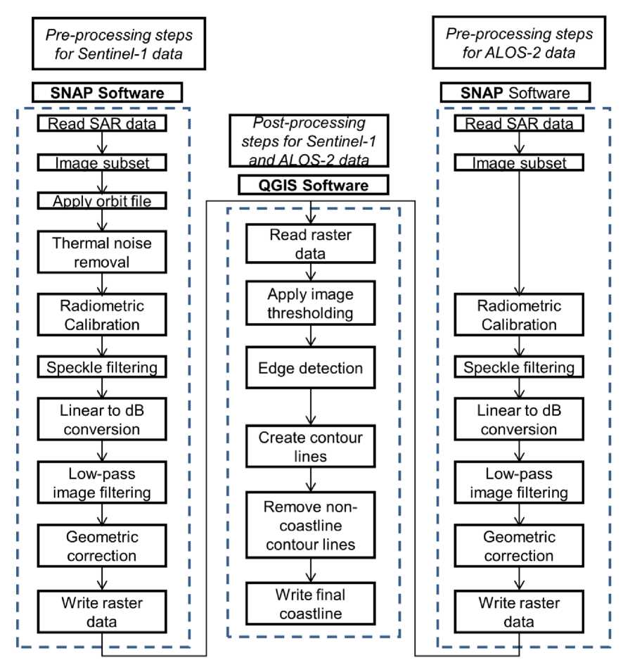
Figure 1. Processing steps in this proposed procedure
-
2.2. Study Area
The study area is Noheji, Kamikita district, Aomori prefecture, Japan, as shown in Figure 2. It is a coastal area located in the inland sea (Mutsu Bay).
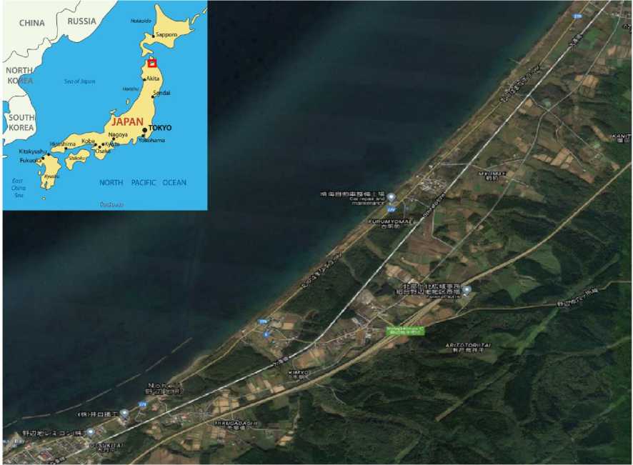
Figure 2. procedure Location of the study area in Noheji, Kamikita district, Aomori prefecture, Japan
This study uses Sentinel-1 and ALOS-2 SAR datasets. The Sentinel-1 data can be downloaded free or at charge from the Copernicus program website (https://scihub.copernicus.eu/dhus/#/home). ALOS-2 data cannot be downloaded for free. The user must purchase the dataset or apply a proposal to get the dataset for free for research usage. The information about the SAR dataset is given in Table 1. Polarization means how the way of Satellite transmits and receives the data. Vertical-Vertical (VV) means the Satellite transmits electromagnetic waves in a vertical vector and receives the reflected electromagnetic waves in a vertical vector. Vertical-Horizontal (VH) means the Satellite transmits electromagnetic waves in vertical vector and receives the reflected electromagnetic waves in horizontal vector. HorizontalHorizontal (HH) means the Satellite transmits electromagnetic waves in a horizontal vector and receives the reflected electromagnetic waves in a horizontal vector.
Sentinel-1 SAR datasets (VV and VH) were taken at once on June 26, 2017, at 17:26 local time. ALOS-2 SAR dataset was taken on June 27, 2017, at 23:31 local time. The observation time difference between Sentinel-1 and ALOS-2 is only one day.
The spatial resolution or the size of one pixel of the Sentinel-1 SAR dataset (VV and VH) is 10 x 10 meters, while ALOS-2 is 3 x 3 meters. It means ALOS-2 is three times higher resolution than the Sentinel-1 SAR dataset (VV and VH).
|
Table 1. SAR dataset used in this study | |
|
Platform |
Observation date Resolution Polarization |
|
Sentinel-1 Sentinel-1 ALOS-2 |
2017-06-26 at 17:26 local time 10 x 10 meters VV 2017-06-26 at 17:26 local time 10 x 10 meters VH 2017-06-27 at 23:31 local time 3 x 3 meters HH |
Figure 3 shows the SAR image before and after low-pass filtering for Sentinel-1 VV polarization. Both images did not show much difference visually. However, from the pixel value histogram, there are many improvements between before and after low-pass filtering. The histogram of the filtering image shows a more apparent distribution than the original image. It makes it easier to distinguish between pixels from the water surface and land surface. This filtered histogram is used to decide the threshold value in the image thresholding step.
Sentinel-1 VV before low-pass filter (image date: 2017-06-26 at 17:26 local time)
(b)
Sentinel-1 W after low-pass filter (image date: 2017-06-26 at 17:26 local time)
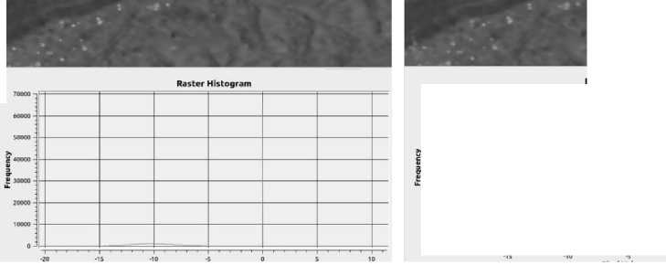
Figure 3. Application of low-pass filter to Sentinel-1 VV: (a) before and (b) after the low-pass filter is applied. The X-axis is the pixel value (in dB), and Y-axis is the frequency of pixel value.
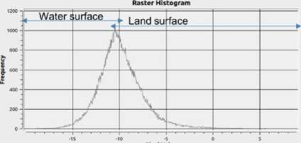
The results of before and after low-pass filtering for Sentinel-VH polarization are presented in Figure 4. Same as in Figure 3, both images did not show much difference visually. From the pixel value histogram, there is much improvement between before and after low-pass filtering. Compared with Sentinel-1 VV polarization, Sentinel-1 VH polarization shows a better histogram. It is because Sentinel-1 VH has a smaller Coefficient of Variation (CV) of pixel value than Sentinel-1 VV. The coefficient of Variation (CV) of the pixel value is one of the parameters to assess SAR data polarization quality. CV can be calculated by:
CV =
standar deviation of pixel value mean of pixel value
(4)
The smaller value of CV is better for coastline extraction. In this case, the CV value for Sentinel-1 VV and VH are 10,78 and 5,24, respectively. Thus, the histogram of the filtered image of Sentinel-1 VH polarization shows an obvious pixel value between water and land surfaces.
Sentinel-1 VH before low-pass filter (image date: 2017-06-26 at 17:26 local time)
Sentinel-1 VH after low-pass filter (image date: 2017-06-26 at 17:26 local time)
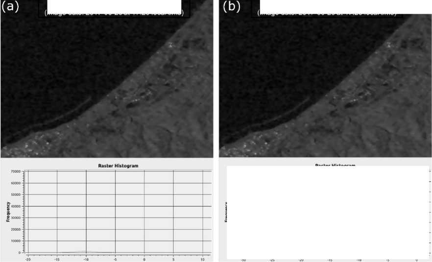
filter is applied. The X-axis is the pixel value (in dB), and Y-axis is the frequency of pixel value.
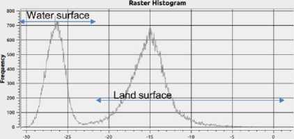
Figure 4. Application of low-pass filter to Sentinel-1 VH: (a) before and (b) after the low-pass
Figure 5 shows ALOS-2 HH polarization results before and after low-pass filtering. ALOS-2 has 3 x 3 meters resolution and provides a detailed SAR image (Fig. 5). The histogram of ALOS-2 after low-pass filtering provides a similar pattern as Sentinel-1 VH (Fig. 4). It shows that ALOS-2 has a better result than Sentinel-1 even though ALOS-2 only uses HH polarization. It is expected that this method can be tested to ALOS-2 HV polarization.
ALOΞ-2 HH before low-pass filter (image date: 2017-06-27 at 23:31 local time)
ALOS-2 HH after low-pass filter (image date: 2017-06-27 at 23:31 local time)
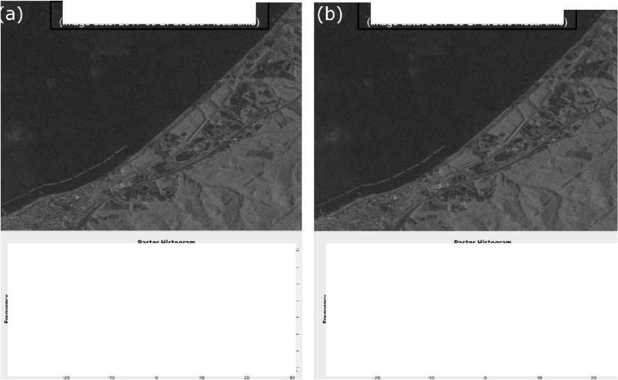
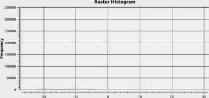
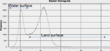
Figure 5. Application of low-pass filter to ALOS-2 HH: (a) before and (b) after the low-pass filter is applied. The X-axis is the pixel value (in dB), and Y-axis is the frequency of pixel value.
Figures 3, 4, and 5 show different histogram patterns (after the low-pass filter is applied) for each dataset. It indicates the ability of each dataset to distinguish between the land surface and water surface. This ability depends on the polarization and resolution of the satellite dataset.
The final coastlines of Sentinel-1 VV, Sentinel-1 VH, and ALOS-2 HH are shown in Fig. 6. In general, ALOS-2 HH provides the best result among those Sentinel-1 ones. The main reason is that the resolution of ALOS-2 is almost three times better than Sentinel-1. However, ALOS-2 is not provided for free. It means not all users can try this method using the ALOS-2 dataset. Furthermore, using Sentinel-1 VH provides a better coastline than Sentinel-1 VV.
The coastline provided by ALOS-2 and Sentinel-1 is slightly different. It is because the observation times between ALOS-2 and Sentinel-1 are different. Sentinel-1 took the data at 17:26 local time, while ALOS-2 took the data one day after at 23:31 local time. The possibility of a tidal effect is strong.
This research focuses on explaining the proposed procedure, and the tidal correction is not applied, and it has become future work to improve the accuracy of detected coastline.
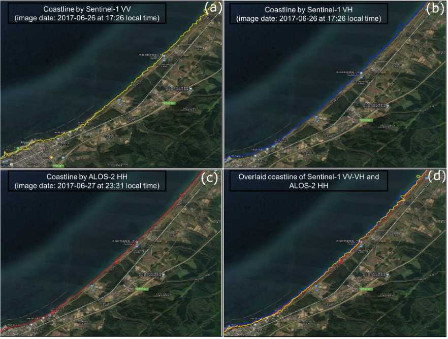
Figure 6. Coastlines generated from SAR data: (a) Sentinel-1 VV, (b) Sentinel-1 VH, (c) ALOS-2 HH, and (d) Overlaid of Sentinel-1 VV-VH and ALOS-2 HH
This research demonstrates the proposed procedure for extracting coastline from the SAR dataset. The detail of the processing steps is explained. The proposed procedure is tested using Sentinel-1 VV, Sentinel-1 VH, and ALOS-2 HH SAR datasets. The results show that a low-pass filtering algorithm can improve the histogram of each SAR dataset. In general, ALOS-2 provides the best coastline among Sentinel-1 ones. It is because ALOS-2 has three times better spatial resolution than Sentinel-1. The coastline provided by ALOS-2 and Sentinel-1 is slightly different. It is because the observation times between ALOS-2 and Sentinel-1 are different. Sentinel-1 took the data at 17:26 local time, and ALOS-2 took the data one day after at 23:31 local time. The possibility of a tidal effect is strong.
For future work, it is recommended to conduct a deep analysis of the effect of the resolution of the satellite dataset on the final results of extracted coastline. It can be done by conducting a comparative study using several satellite datasets in different resolutions. In addition, it is a good chance to test this procedure with the ALOS-2 HV SAR dataset. ALOS-2 HV SAR dataset is expected to provide a better result than ALOS-2 HH. For a more advanced comparison between coastline provided by ALOS-2 and Sentinel-1, it is better to apply Digital Shoreline Analysis System (DSAS) for those results. This time DSAS is not applied because DSAS is an add-on of ArcGIS software (commercial license).
References
-
[1] M. J. F. Stive et al., "Variability of shore and shoreline evolution," Coastal Engineering,
vol. 47, pp. 211–235, 2002, [Online]. Available: www.elsevier.com/locate/coastaleng
-
[2] G. Anfuso, E. Pranzini, and G. Vitale, "An integrated approach to coastal erosion problems
in northern Tuscany (Italy): Littoral morphological evolution and cell distribution," Geomorphology, vol. 129, no. 3–4, pp. 204–214, Jun. 2011, doi:
10.1016/j.geomorph.2011.01.023.
-
[3] R. M. Sorensen, Basic Coastal Engineering, Third edit. Springer Science & Business
Media, 2005.
-
[4] T. A. Łabuz, "Environmental Impacts—Coastal Erosion and Coastline Changes," pp. 381–
-
396, 2015, doi: 10.1007/978-3-319-16006-1_20.
-
[5] A. Spinosa, A. Ziemba, A. Saponieri, V. D. Navarro-Sanchez, L. Damiani, and G. el Serafy,
"Automatic extraction of shoreline from satellite images: A new approach," in 2018 IEEE International Workshop on Metrology for the Sea; Learning to Measure Sea Health Parameters, MetroSea 2018 - Proceedings, Mar. 2019, pp. 33–38. doi:
10.1109/MetroSea.2018.8657864.
-
[6] I. Sekovski, F. Stecchi, F. Mancini, and L. del Rio, "Image classification methods applied
to shoreline extraction on very high-resolution multispectral imagery," International Journal of Remote Sensing, vol. 35, no. 10, pp. 3556–3578, 2014, doi:
10.1080/01431161.2014.907939.
-
[7] T. Y. Shyu, H. C. Yeh, and C. C. Liu, "Mapping of a boundary line from remote sensing:
An applied case study on Little Okinawa Island," International Journal of Remote Sensing, vol. 33, no. 23, pp. 7599–7608, 2012, doi: 10.1080/01431161.2012.685987.
-
[8] L. C. Chen and J. Y. Rau, "Detection of shoreline changes for tideland areas using multi
temporal satellite images," International Journal of Remote Sensing, vol. 19, no. 17, pp. 3383–3397, 1998, doi: 10.1080/014311698214055.
-
[9] F. S. Kawakubo, R. G. Morato, R. S. Nader, and A. Luchiari, "Mapping changes in
coastline geomorphic features using landsat TM and ETM+ imagery: Examples in southeastern Brazil," International Journal of Remote Sensing, vol. 32, no. 9, pp. 2547– 2562, 2011, doi: 10.1080/01431161003698419.
-
[10] C. Wang, J. Zhang, and Y. Ma, "Coastline interpretation from multispectral remote sensing images using an association rule algorithm," International Journal of Remote Sensing, vol. 31, no. 24, pp. 6409–6423, 2010, doi: 10.1080/01431160903413739.
-
[11] A. Ahmed, F. Drake, R. Nawaz, and C. Woulds, "Where is the coast? Monitoring coastal land dynamics in Bangladesh: An integrated management approach using GIS and remote sensing techniques," Ocean and Coastal Management, vol. 151, no. July, pp. 10–24, 2018, doi: 10.1016/j.ocecoaman.2017.10.030.
-
[12] O. A. Dada, A. O. Agbaje, R. B. Adesina, and Y. A. Asiwaju-Bello, "Effect of coastal land use change on coastline dynamics along the Nigerian Transgressive Mahin mud coast," Ocean and Coastal Management, vol. 168, no. April 2018, pp. 251–264, 2019, doi: 10.1016/j.ocecoaman.2018.11.014.
-
[13] S. Patel, E. Shah, P. Jayaprasad, and M. E. James, "Changes in Antarctic coastline between 1997 and 2016 using RADARSAT and MODIS data," International Journal of Remote Sensing, vol. 41, no. 4, pp. 1389–1414, Feb. 2019, doi: 10.1080/01431161.2019.1667550.
-
[14] M. Modava and G. Akbarizadeh, "Coastline extraction from SAR images using spatial fuzzy clustering and the active contour method," International Journal of Remote Sensing, vol. 38, no. 2, pp. 355–370, Jan. 2017, doi: 10.1080/01431161.2016.1266104.
-
[15] E. Ferrentino, F. Nunziata, and M. Migliaccio, "Full-polarimetric sar measurements for coastline extraction and coastal area classification," International Journal of Remote Sensing, vol. 38, no. 23, pp. 7405–7421, Dec. 2017, doi:
10.1080/01431161.2017.1376128.
-
[16] X. Ding and X. Li, "Shoreline movement monitoring based on SAR images in Shanghai, China," International Journal of Remote Sensing, vol. 35, no. 11–12, pp. 3994–4008, 2014, doi: 10.1080/01431161.2014.916480.
-
[17] Y. Ouyang, J. Chong, and Y. Wu, "Two coastline detection methods in synthetic aperture radar imagery based on level set algorithm," International Journal of Remote Sensing, vol. 31, no. 17, pp. 4957–4968, 2010, doi: 10.1080/01431161.2010.485142.
-
[18] S. Zollini, M. Alicandro, M. Cuevas-González, V. Baiocchi, D. Dominici, and P. M. Buscema, "Shoreline extraction based on an active connection matrix (ACM) image enhancement strategy," Journal of Marine Science and Engineering, vol. 8, no. 1, 2020, doi: 10.3390/jmse8010009.
-
[19] C. Dai, I. M. Howat, E. Larour, and E. Husby, "Coastline extraction from repeat high resolution satellite imagery," Remote Sensing of Environment, vol. 229, no. April, pp. 260– 270, 2019, doi: 10.1016/j.rse.2019.04.010.
-
[20] R. Gens, "Remote sensing of coastlines: Detection, extraction and monitoring," International Journal of Remote Sensing, vol. 31, no. 7. Taylor and Francis Ltd., pp. 1819– 1836, 2010. doi: 10.1080/01431160902926673.
-
[21] R. Pelich, M. Chini, R. Hostache, P. Matgen, and C. Lopez-Martinez, "Coastline Detection Based on Sentinel-1 Time Series for Ship- and Flood-Monitoring Applications," IEEE Geoscience and Remote Sensing Letters, pp. 1–5, 2020, doi: 10.1109/lgrs.2020.3008011.
-
[22] M. Schmitt, G. Baier, and X. X. Zhu, "Potential of nonlocally filtered pursuit monostatic TanDEM-X data for coastline detection," ISPRS Journal of Photogrammetry and Remote Sensing, vol. 148, no. July 2018, pp. 130–141, 2019, doi: 10.1016/j.isprsjprs.2018.12.007.
185
Discussion and feedback