Forecasting of Sea Level Time Series using RNN and LSTM Case Study in Sunda Strait
on
LONTAR KOMPUTER VOL. 12, NO. 3 DECEMBER 2021
DOI : 10.24843/LKJITI.2021.v12.i03.p01
Accredited Sinta 2 by RISTEKDIKTI Decree No. 30/E/KPT/2018
p-ISSN 2088-1541
e-ISSN 2541-5832
Forecasting of Sea Level Time Series using RNN and LSTM Case Study in Sunda Strait
Annas Wahyu Ramadhana1, Didit Adytiaa2, Deni Saepudina3, Indwiartia4, Semeidi Husrinb5, Adiwijayaa6
a
b
School of Computing, Telkom University Bandung, Indonesia 1annaswramadhan@student.telkomuniversity.ac.id 2adytia@telkomuniversity.ac.id(Corresponding author) 3denisaepudin@telkomuniversity.ac.id 4indwiarti@telkomuniversity.ac.id 6adiwijaya@telkomuniversity.ac.id
Marine Research Centre, Ministry of Marine Affairs and Fisheries of Indonesia Jakarta, Indonesia 5s.husrin@kkp.go.id
Abstract
Sea-level forecasting is essential for coastal development planning and minimizing their significant consequences in coastal operations, such as naval engineering and navigation. Conventional sea level predictions, such as tidal harmonic analysis, do not consider the influence of non-tidal elements and require long-term historical sea level data. In this paper, two deep learning approaches are applied to forecast sea level. The first deep learning is Recurrent Neural Network (RNN), and the second is Long Short Term Memory (LSTM). Sea level data was obtained from IDSL (Inexpensive Device for Sea Level Measurement) at Sebesi, Sunda Strait, Indonesia. We trained the model for forecasting 3, 5, 7, 10, and 14 days using three months of hourly data in 2020 from 1st May to 1st August. We compared forecasting results with RNN and LSTM with the results of the conventional method, namely tidal harmonic analysis. The LSTM’s results showed better performance than the RNN and the tidal harmonic analysis, with a correlation coefficient of R2 0.97 and an RMSE value of 0.036 for the 14 days prediction. Moreover, RNN and LSTM can accommodate non-tidal harmonic data such as sea level anomalies.
Keywords: Sea Level, Forecasting, Deep Learning, RNN, LSTM
Information on the sea level is necessary for the operation of ports, in particular, for the scheduling of naval transportation and the port services operation [1]. Ships with deep draft depend on the sea level forecasting for their navigation in a shallow coastal area. Moreover, historical data on the sea level is vital for the planning of coastal and offshore buildings, and the sea level prediction is necessary during the construction phase of the structures [2]. Another importance of predicting sea level is to gather information on climate change how likely the rise of sea level is in the future so that we can minimize the consequent, especially in a coastal area such as flooding [3]. The sea level consists of two general elements, tidal and non-tidal elements. The dominant forces shaping the sea level are the tidal elements because tidal is the most stable pattern in oceanographic [4]. The non-tidal elements come from wind or other occurrences that are affecting the sea level [5]. Tidal harmonic analysis (THA) is a conventional way to forecast sea level. THA assumes sea
level as a superposition of harmonic components or tidal representatives. Typically, using Least Square Estimation (LSE), the tidal components in a given area can be reliably calculated using the measured sea level. However, the forecasted sea level is the tidal parts only since THA cannot predict the non-tidal components. Another major downside, THA needs long historical sea level data to extract all tidal elements.
Various attempts proposed to improve the accuracy of the THA method for predicting the sea level, such as using multivariate least-square harmonic estimation [6] and combining the LSE method with the Inaction Method (IM) [7]. Moreover, there is also another approach for predicting sea-level namely ARIMA (Autoregressive Integrated Moving Average) [8], SARIMA (Seasonal Autoregressive Integrated Moving Averaged) [9], and Holtz-Winters Exponential Smoothing [10]. The prediction performance from ARIMA, SARIMA, and Holtz-Winters for seven prediction days measured by RMSE are 0.226, 0.155, and 0.134, respectively. These results offer a challenge to finding a better predictive model. ARIMA, SARIMA, and Holt-Winter approaches are methods based on time series analysis. Machine learning approaches such as ANN (Artificial Neural Network) to forecast sea-level is discussed in [11] where ANN is applied to predict sea level anomalies. In 2018, Imani et al. [12] applied relevance vector machine models and extreme learning machines to predict sea-level. Rizkina et al. [13] in 2019 compared the nonlinear autoregressive (NAR) neural network and tidal harmonic analysis to obtain a short-term prediction of sea level in Semarang. Using the NAR method, they obtain prediction with an R-value of 0.9566 and an RMSE value of 0.0736.
This research aims to investigate a reliable sea-level prediction approach that needs only reasonably short-term historical data. Sea level prediction is carried out by applying the Recurrent Neural Network (RNN) and Long Short-Term Memory (LSTM), two popular deep learning methods. RNN is a type of neural network designed to handle sequential data. Not only suitable for solving classification problems in Natural Language Problem (NLP), the RNN is also suitable for predicting time series data. However, RNN often encounters problems such as vanishing the gradient, where the loss function decreases exponentially. It interferes with the learning process. LSTM is an improvement RNN to avoid this problem. LSTM architecture consists of a memory cell, input gate, forget gate, and output gate. As a study area, we chose the Sebesi station in Sunda Strait, Indonesia. Sea level data comes from measurements by IDSL or Inexpensive Device for Sea Level measurement. The RNN and LSTM in predicting the sea level is then compared to the traditional approach using THA.
Figure 1 shows our research methodology. The study utilizes the sea level data obtained from the IDSL at Sebesi station in Sunda Strait, Indonesia. The raw data is pre-processed to remove noises as well as to fill in missing data. The data set is then separated into training also testing data and then tested for three forecasting methods, the traditional THA and the deep learning methods using the RNN and LSTM. We performed several forecasting scenarios based on the length of days to forecast for 3, 5, 7, 10, and 14 days. The prediction results from these three methods are then compared qualitatively and quantitatively. The performance is measured using the correlation coefficients (R2) together with the Root Mean Square Error (RMSE). These steps in the methodology of this paper are explained in more detail in Figure 1.
The data are collected from a sea-level measurement device called IDSL (Inexpensive Device for Sea Level measurement). The IDSL is a joint effort between the European Commission’s Joint Research Centre, The Marine Research Centre of MMAF, and The Indonesia Society of Tsunami Experts (IATSI). The station supports the tsunami early warning system in the Sunda Strait due to its proximity to the Krakatau Volcano that generated the tsunami in 2018 [14]. The Sebesi station was selected for IDSL due to its important location as a tourism destination and community livelihoods. Monitoring of sea levels due to global climate change is also vital for sealevel rise risk mitigation. The location of Sebesi Station is between the lines 5° 56’ 9.7692" South Latitude and 105° 30’ 43.5816" East Longitude as shown in Figure 2.
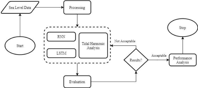
Figure 1. Research methodology in this study.
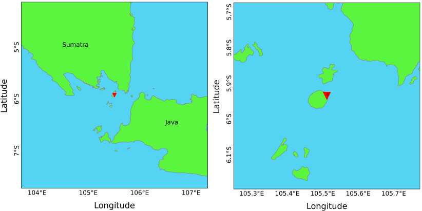
Figure 2. Location of tidal buoy in Sebesi.
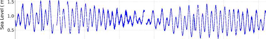
The sea level data from the IDSL is recorded initially every 20 seconds. It is unnecessary to use detailed temporal spacing data for sea-level forecasting since they include unnecessary harmonic components, especially high frequencies. Instead, we use hourly data for sea level forecasting. Moreover, the measured sea level data contained missing values, which will lead to a problem for the forecasting process by using a deep learning approach. To that end, the original 20s temporal data is transformed into hourly data by calculating the average.
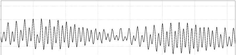
In this paper we use 3.5 months data, i.e. 1th May - 15th August 2020. The original 20 s temporal data is shown in the top of Figure 3, whereas the hourly sea level data is depicted in the middle of Figure 3. The missing values in the original data are filled with interpolated data shown in the lower plot of Figure 3.
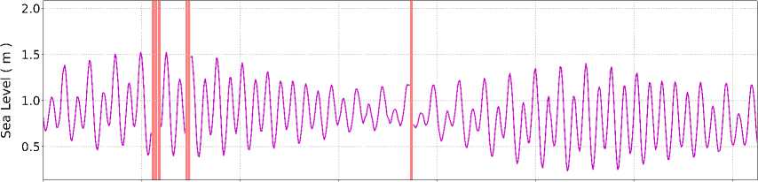
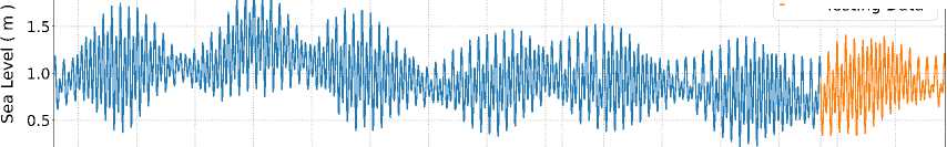
The preprocessed data is separated into training and testing data as depicted by Figure 4. We use three months of sea level data, 1th May - 31th July 2020 for training to forecast 3, 5, 7, 10, and 14 days ahead.
A brief explanation related to the three forecasting methods, the classical Tidal Harmonic Analysis (THA), Recurrent Neural Network (RNN) as well as the Long Short Term Memory (LSTM) are described in the following subsection.
Original Sea Level Data at Sebesi
2.0
3,ul-01 Jul-05 Jul-09 Jul-13 Jul-17 Jul-21 Jul-25 Jul-29
Time ( Month - Day ) - 2020
Hourly Sea Level Data at Sebesi
Jul-Ol
Jul-05
Jul-09
Jul-13
Jul-17
Jul-21
Jul-25
Jul-29
Time ( Month - Day ) - 2020
Preprocessed Sea Level Data at Sebesi
2.0
E
1.5
1.0
φ
0.5
φ
UO
Jul-05
Jul-09
Jul-13
Jul-17
Jul-21
Jul-25
Jul-29
Time ( Month - Day ) - 2020
Bul-Ol
Figure 3. Time series of sea level data at Sebesi from 1th - 30th July 2020: Original data (upper plot), hourly data (middle plot), and interpolated hourly data (lower plot). The missing data are indicated by red area in the middle plot.
As stated in [15], the sea level is mainly generated by tidal waves, which are strongly influenced by the moon and the sun. The tide is affected by the relative astronomical location of the earth with the moon and the sun. Changes in the astronomical location lead to the rising and dropping of the sea level. These astronomical forces that shape the tide could be considered as a summation of harmonic components, which is the core principle of the Tidal Harmonic Analysis (THA) method [6, 7]. This fact makes the tide the most predictable oceanographic physical phenomenon, especially compared to wind and waves [4]. As a result, the tide can be expressed as (1)
N
h(t) = ho + y fiHi cos(ωit - gi). (1)
i=1
Here, h0 is the mean of sea level or MSL, fi is the node factor, Hi is the ith amplitude component of the tidal component-i, ωi, and gi are the the ith tidal constituent and its phase, respectively. High and low tides can be calculated by searching the critical value of the formula (1), by calculating the first derivative of the formula, equated to zero as in equation (2). Nevertheless, the equation (1)
Training & Testing Sea Level Data at Sebesi
2.0
---- Training Data Testing Data
0.0
Ju∣
Aug
Jun 2020
Time ( Month - Day ) - 2020
Figure 4. Sea level data splitting, training data (1 May - 31 July 2020 or 80 %, indicated by blue line) and testing data (1-15 August 2020 or 20 %, indicated by yellow line).
cannot capture the variation in the peak tide since the peak of superposition of harmonic waves in the equation (1) are constant and appear periodically.
N
- ∑2 fiHi sin(ωit - Si) = 0.
(2)
i=1
There is no analytic solution for the equation (2). The parameters Hi , fi , ωi , and gi are estimated using the Least Square Estimation (LSE) method with measured sea level as the reference in many tidal harmonic analysis methods [16]. As a consequence of the THA approach, the THA method cannot predict non-tidal elements at sea level. Moreover, the THA method requires a relatively long historical sea level data set to correctly describe the low frequencies component of the sea level.
RNN is a family of artificial neural network (ANN) architecture that processes interrelated repetitive input typically in sequential data, including time-series data. The RNN differs from the traditional Neural Network. Each processing produced in the RNN is influenced by the current input and an internal state resulting from the previous input processing. When the RNN makes a decision, the time step t - 1 can influence the decision to be taken at time step t [17].
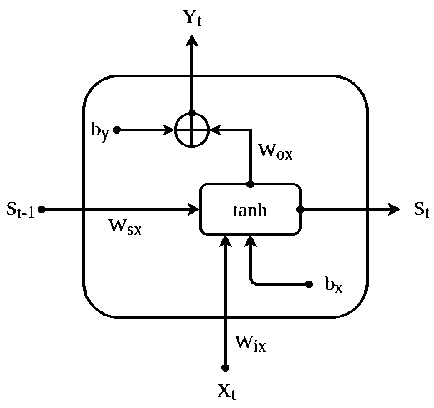
Figure 5. The architecture of Recurrent Neural Network (RNN).
The RNN is a method commonly used for forecasting problems. In [18], the RNN is used for forecasting wind speed, where they also compare the method with the ARIMA model. In [19], the RNN is used for forecasting for electricity consumption in medium-to-long-term, where they conclude that the RNN produces better prediction than the three-layer multilayer perceptron model.
The architecture of the RNN can be illustrated as in Figure 5. Here, for each time step t, the state St is calculated from the input Xt and the prior state St-1 by following the formula (3)
St = tanh(WiχX t + W sχSt-i + bχ).
(3)
Here, Wix and Wsx are the weight matrix at input and hidden layer respectively, and bx denotes the bias. The function tanh(x) is an activation function that is defined by the following formula
tanh(x) =
e
-x
ex + e-x,
(4)
where the range of function tanh(x) is from -1 to 1.
The output value Yt is given by the following formula
Yt = W oxS t + by,
(5)
where Yt denotes the output, Wox is the weighted matrix at output layer, St is the states, and by is the bias.
LSTM was initiated by Hochreiter and Schmidhuber [20]. It is an improved version of RNN where LSTM is equipped with a memory cell that could reserve information for a long time. Vanishing and exploding gradient problems are problems in the RNN that fail to capture long-term dependencies, thereby reducing the accuracy of a prediction on RNN [21]. Meanwhile, the LSTM could store or discard data since each neuron has several gates that regulate the memory of each neuron. Figure 6 shows the layout of the gates of LSTM.
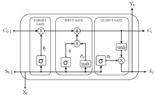
Figure 6. The architecture of LSTM.
In LSTM there are three gates, namely ft, it, and ot as shown in Figure 6. Gate ft is the forget gate, it is the input gate, and ot is the output gate [2].
The first step in assembling the LSTM is to differentiate the necessary and unnecessary data in the first gate (forget-gate). A sigmoid function (6) defines this process. If the value of the sigmoid function is 0 then the data will be discarded. If the value is 1 then the data will be updated or passed through. Xt is the current input value and St-1 is the hidden state of the prior value. W and b are coefficients where their values are determined from the training process.
ft = σ(W fχ X t + W fsS t-i + bf)
(6)
The next process is in the input gate. The input gate controls how many states from the current input will pass through. The output is determined by the sigmoid function (7) in the first layer, and the hyperbolic tangent function (8) in the second layer, where the value of the cell state Ct is defined in equation (9).
it = σ(Wχ X t + W is S t-i + b i).
(7)
(8)
(9)
Ct = tanh(W cx X t + W cs S - + b c).
C t = f t × c t-1 + i t × Ct.
And the final gate unit component is the output gate, which decides the internal state forward and the cell state or memory cell to forward old information with additional new information to the next cell state.
(10)
(11)
ot = σ(Woχ X t + W os S t—i + b o) St = ot × tanh(ct).
By following the calculation at the output gate as defined in equation (10), the output value, namely the cell state value Ct will be forwarded for the next memory cell calculation, and the current hidden state St , will be generated using equation (8).
In this evaluation section, the optimal model search process is carried out, especially for using deep learning models, namely RNN and LSTM. In searching for the optimal model for this deep learning model, some stages are carried out. The first is searching for the optimal model by calculating the scoring metric using the Correlation Coefficient and Mean Square Error. If in the first stage of the search for the model the best model is obtained, then in the second stage by finding the optimal number of lookbacks from the deep learning model by taking into account the computational time in the training process itself, by using these two stages the model with the best results is obtained.
The performance of both RNN and LSTM is evaluated by calculating the Root Mean Square Error (RMSE) and R2 to see which one is better. The RMSE is a formula for measuring the average error and is written as follows.
RMSE =
1 N
N ∑y - yi)2.
(12)
In equation (12), N is the total value of input data, yi is the output of the prediction value and yi is the target value [22].
The coefficient of determination R2 is a useful quantitative usually used to measure how well the output of a model in predicting the target. Values of R2 are between 0 and 1 [23]. The R2 is defined as follows in equation (13-15),
R2
SSR
(13)
(14)
SST ,
N
SSR = X(yi - yi)2,
where SSR is the Sum of Squared Residuals and SST is the Sum of Squared Total, where yi is the observed value, N is the amount of data, and y is the value of the prediction.
Mean Bias Error (MBE) is useful to calculate average bias in the prediction and defined as [24]
1 N
(16)
MBE = n ∑(⅛ - yi)
A positive MBE means that the predictions are overestimating, and a negative MBE means an underestimation.
As explained in the previous section, we use the sea level data from 1th May - 15th August 2020 at Sebesi Station. Using three months of sea level data for training data for the Tidal Harmonic Analysis, RNN, and LSTM model, predict the next 3 to 14 days ahead. Based on Table 1, the LSTM model shows better performance in predicting sea-level compared to the Tidal Harmonic Analysis and RNN model.
Table 1. Prediction Result Of THA, RNN and LSTM
|
Prediction (Days) |
THA |
RNN |
LSTM | ||||||
|
R2 |
RMSE |
MBE |
R2 |
RMSE |
MBE |
R2 |
RMSE |
MBE | |
|
3 |
0.8132 |
0.1214 |
-0.1127 |
0.9595 |
0.0580 |
0.0504 |
0.9795 |
0.0413 |
0.0353 |
|
5 |
0.8398 |
0.1173 |
-0.1096 |
0.9663 |
0.0547 |
0.0474 |
0.9827 |
0.0392 |
0.0326 |
|
7 |
0.8675 |
0.1082 |
-0.0984 |
0.9681 |
0.0538 |
0.0466 |
0.9827 |
0.0394 |
0.0326 |
|
10 |
0.8799 |
0.0976 |
-0.0856 |
0.9686 |
0.0496 |
0.0426 |
0.9818 |
0.0377 |
0.0306 |
|
14 |
0.8721 |
0.0905 |
-0.0790 |
0.9631 |
0.0479 |
0.0408 |
0.9782 |
0.0369 |
0.0295 |
Based on Table 1, the RMSE value of RNN is smaller than the RMSE value of THA for all prediction days. It shows that prediction with RNN provides a closer estimate than THA. The result is consistent with the value of the coefficient deterministic R2 . The coefficient deterministic of RNN is closer to one than THA. It means that the predicted results of RNN have a better match with the original data than THA. However, prediction with LSTM gives better results than RNN for all prediction days, both measured by RMSE and by R2 . As an improved version of RNN, the performance of LSTM is better than RNN due to its ability to handle information for a long time that overcomes vanishing and exploding gradient problems in RNNs. By analyzing the length of the prediction day, it can be seen that the longer the prediction day, the better the prediction result. On longer prediction days, prediction errors will be more distributed. The MBE values of THA are negatives for all prediction days. It means the THA predictions are underestimating. The MBE of RNN and LSTM are positives for all prediction days. It means that their predictions are overestimating. The MBE of LSTM is smaller than RNN’s. Overall, prediction with LSTM with 14 prediction days gives the best results.
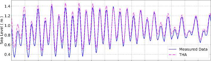
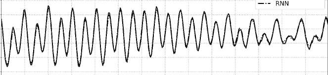
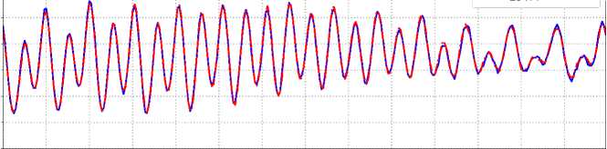
Qualitative comparison between the prediction for 14 days with Tidal Harmonic Analysis, RNN, and LSTM is shown in Figure 7. Based on Figure 7 we can see that the prediction results using THA cannot accurately estimate the sea level around the top and bottom. The predictive graph of THA is periodic and very well accommodates the tidal component of the sea level but fails to accommodate the non-tidal element that affects the sea level. The THA model only considers the influence of tidal components such as the tractive force of the sun, moon, and other astronomical objects. The tidal component contributions are represented as a superposition of trigonometric functions, as written in equation (1). Other components such as the effects of wind, waves, and global warming have not been accommodated in the THA model. Even though the influence of these components is not dominant, the effect is significant, especially at the top and bottom. Prediction results using deep learning estimate sea levels more accurately, including around the
top and bottom of the sea level. These predictions are also better than the previous prediction methods using ARIMA, SARIMA, and Holt-Winters for testing with seven prediction days which give RMSE 0.226, 0.155, and 0.134, respectively [10]. The RMSE values of RNN and LSTM for seven prediction days are0.054 and 0.039, respectively.
Prediction by THA: 14 Days Forecast
1 2 3 4 5 6 7 8 9 10 11 12 13 14
Time ( Hours )
1.75
Prediction by RNN: 14 Days Forecast
--- Measured Data
2
3
4
5
6
7 8 9
Time ( day )
10 11 12 13 14
1.50
^ 1.25 E
_ ι.oo φ
.I! 0.75
ro
Φ
ω 0.50
0.25
o.oo;-
Prediction by LSTM: 14 Days Forecast
Measured Data LSTM
0.75
0.25
φ φ
φ in 0.50
~ 1.25 E
T 1.00
2
3
4
5
6
7 8 9
Time ( Day )
10 11 12 13 14
1.75
1.50
0.001
Figure 7. Tidal Harmonic Analysis (upper plot), RNN (middle plot), LSTM (lower plot) for 14 days forecast at Sebesi.
We predict sea level using deep learning approaches, the Recurrent Neural Network together with Long Short-Term Memory. As training data, we use three months time series of sea level data to train the model to predict 3, 5, 7, 10, and 14 days. We conducted a prediction with Tidal Harmonic Analysis, RNN, and LSTM method. All methods we used can predict with reasonably good performance and follow the measured value of the buoy. However, the deep learning approach shows better prediction than the Tidal Harmonic Analysis. Moreover, LSTM shows performance improvement in predicting long-term sea-level data (14 days) with a R2 value of 0.97 and RMSE value of 0.036. These results are better than RNN with a R2 value of 0.96 and the RMSE value of 0.047.
References
-
[1] A.-L. Balogun and N. Adebisi, “Sea level prediction using arima, svr and lstm neural network: assessing the impact of ensemble ocean-atmospheric processes on models’ accuracy,” Ge-omatics, Natural Hazards and Risk, vol. 12, no. 1, pp. 653–674, 2021.
-
[2] X.-H. Le, H. V. Ho, G. Lee, and S. Jung, “Application of long short-term memory (lstm) neural network for flood forecasting,” Water, vol. 11, no. 7, p. 1387, 2019.
-
[3] G. Griggs, “Rising seas in california—an update on sea-level rise science,” in World Scientific Encyclopedia of Climate Change: Case Studies of Climate Risk, Action, and Opportunity Volume 3. World Scientific, 2021, pp. 105–111.
-
[4] G. D. Egbert and R. D. Ray, “Tidal prediction,” Journal of Marine Research, vol. 75, no. 3, pp. 189–237, 2017.
-
[5] C. Y. Zhang, “Non-Tidal Water Level Variability in Lianyungang Coastal Area,” Advanced Materials Research, vol. 610-613, pp. 2705–2708, Dec. 2012. [Online]. Available: https://www.scientific.net/AMR.610-613.2705
-
[6] A. Amiri-Simkooei, S. Zaminpardaz, and M. Sharifi, “Extracting tidal frequencies using multivariate harmonic analysis of sea level height time series,” Journal of Geodesy, vol. 88, no. 10, pp. 975–988, 2014.
-
[7] S. Li, L. Liu, S. Cai, and G. Wang, “Tidal harmonic analysis and prediction with least-squares estimation and inaction method,” Estuarine, Coastal and Shelf Science, vol. 220, pp. 196– 208, 2019.
-
[8] Y. K. Purba, D. Saepudin, and D. Adytia, “Prediction of sea level by using autoregressive integrated moving average (arima): Case study in tanjung intan harbour cilacap, indonesia,” in 2020 8th International Conference on Information and Communication Technology (ICoICT). IEEE, 2020, pp. 1–5.
-
[9] R. Tulus, D. Adytia, N. Subasita, and D. Tarwidi, “Sea level prediction by using seasonal autoregressive integrated moving average model, case study in semarang, indonesia,” in 2020 8th International Conference on Information and Communication Technology (ICoICT). IEEE, 2020, pp. 1–5.
-
[10] D. S. Wibowo, D. Adytia, and D. Saepudin, “Prediction of tide level by using holtz-winters exponential smoothing: Case study in cilacap bay,” in 2020 International Conference on Data Science and Its Applications (ICoDSA). IEEE, 2020, pp. 1–5.
-
[11] S. Nitsure, S. Londhe, and K. Khare, “Prediction of sea water levels using wind information and soft computing techniques,” Applied Ocean Research, vol. 47, pp. 344–351, 2014.
-
[12] M. Imani, H.-C. Kao, W.-H. Lan, and C.-Y. Kuo, “Daily sea level prediction at chiayi coast, taiwan using extreme learning machine and relevance vector machine,” Global and planetary change, vol. 161, pp. 211–221, 2018.
-
[13] M. A. Rizkina, D. Adytia, and N. Subasita, “Nonlinear autoregressive neural network models for sea level prediction, study case: In semarang, indonesia,” in 2019 7th International Conference on Information and Communication Technology (ICoICT). IEEE, 2019, pp. 1–5.
-
[14] A. Annunziato, G. Prasetya, and S. Husrin, “Anak krakatau volcano emergency tsunami early warning system.” Science of Tsunami Hazards, vol. 38, no. 2, 2019.
-
[15] P. Schureman, Manual of harmonic analysis and prediction of tides. Washington, D.C.: United States Government Printing Office, 1958.
-
[16] S. Cox, “Theory of the Harmonic Model of Tides · sam-cox/pytides Wiki.” [Online]. Available: https://github.com/sam-cox/pytides
-
[17] W. Kong, Z. Y. Dong, Y. Jia, D. J. Hill, Y. Xu, and Y. Zhang, “Short-term residential load forecasting based on lstm recurrent neural network,” IEEE Transactions on Smart Grid, vol. 10, no. 1, pp. 841–851, 2017.
-
[18] K. Sandhu, A. R. Nair et al., “A comparative study of arima and rnn for short term wind speed forecasting,” in 2019 10th International Conference on Computing, Communication and Networking Technologies (ICCCNT). IEEE, 2019, pp. 1–7.
-
[19] A. Rahman, V. Srikumar, and A. D. Smith, “Predicting electricity consumption for commercial and residential buildings using deep recurrent neural networks,” Applied energy, vol. 212, pp. 372–385, 2018.
-
[20] S. Hochreiter and J. Schmidhuber, “Long short-term memory,” Neural computation, vol. 9, no. 8, pp. 1735–1780, 1997.
-
[21] Z. Zhao, W. Chen, X. Wu, P. C. Chen, and J. Liu, “Lstm network: a deep learning approach for short-term traffic forecast,” IET Intelligent Transport Systems, vol. 11, no. 2, pp. 68–75, 2017.
-
[22] J. Zhao, Y. Fan, and Y. Mu, “Sea level prediction in the yellow sea from satellite altimetry with a combined least squares-neural network approach,” Marine geodesy, vol. 42, no. 4, pp. 344–366, 2019.
-
[23] M. Lydia, S. S. Kumar, A. I. Selvakumar, and G. E. P. Kumar, “Wind resource estimation using wind speed and power curve models,” Renewable Energy, vol. 83, pp. 425–434, 2015.
-
[24] R. Pal, “Chapter 4 - validation methodologies,” in Predictive Modeling of Drug Sensitivity, R. Pal, Ed. Academic Press, 2017, pp. 83–107. [Online]. Available: https://www.sciencedirect.com/science/article/pii/B978012805274700004X
140
Discussion and feedback