Helmet Monitoring System using Hough Circle and HOG based on KNN
on
LONTAR KOMPUTER VOL. 12, NO. 1 APRIL 2021
DOI : 10.24843/LKJITI.2021.v12.i01.p02
Accredited Sinta 2 by RISTEKDIKTI Decree No. 30/E/KPT/2018
p-ISSN 2088-1541
e-ISSN 2541-5832
Helmet Monitoring System using Hough Circle and HOG based on KNN
Rachmad Jibril Aa1, Fitri Utaminingruma2, Agung Setia Budia3
aFaculty of Computer Science, University of Brawijaya, Malang, Indonesia
Malang 65141, Fax +62 0341-565420
2f3_ningrum@ub.ac.id (Corresponding author) 3agungsetiabudi@ub.ac.id
Abstract
Indonesian citizens who use motorized vehicles are increasing every year. Every motorcyclist in Indonesia must wear a helmet when riding a motorcycle. Even though there are rules that require motorbike riders to wear helmets, there are still many motorists who disobey the rules. To overcome this, police officers have carried out various operations (such as traffic operation, warning, etc.). This is not effective because of the number of police officers available, and the probability of police officers make a mistake when detecting violations that might be caused due to fatigue. This study asks the system to detect motorcyclists who do not wear helmets through a surveillance camera. Referring to this reason, the Circular Hough Transform (CHT), Histogram of Oriented Gradient (HOG), and K-Nearest Neighbor (KNN) are used. Testing was done by using images taken from surveillance cameras divided into 200 training data and 40 testing data obtained an accuracy rate of 82.5%.
Keywords: Machine learning, Helmet detection, Histogram of an oriented gradient, K-nearest neighbor, Circular hough transform
Motorized vehicles are one type of transportation used in many parts of the world, especially motorbikes. In Indonesia, the number of people has been using motorbikes was increasing. Based on Police Headquarters data in 2013, the number of motorbikes in Indonesia ware 84,732,652 units, a large number of motorbikes caused a high number of traffic accidents involving motorcycles. In 2013 there were 119,560 motorbikes involved in the accident. Referring to the number of an accident has been recorded the total fatalities reached 26,416 (National Police Headquarters)[1].
There are several factors that cause accidents, namely human factors, vehicle factors, and environmental factors[2]. These factors are related to each other, but human factors are the biggest cause of accidents. This is indicated by the records of the National Police Headquarters in 2010-2016, which showed 70% of the causes of accidents were human factors. Many human factors also resulted in the loss of lives. To overcome this, police officers have carried out various operations (such as traffic operation, warning, etc.). This is not effective because of the number of police officers available, and the probability of police officers make mistakes when detecting violations that might be caused due to fatigue.
Over the past few years, many attempts have been made to analyze traffic, including vehicle detection and classification and helmet detection. Modern traffic systems usually use computer vision algorithms, such as background and foreground image detection for the segmentation of moving objects. The use of computer vision algorithms can be applied to the results of video captured by a surveillance camera that is installed on a crossroad or a large road.
Previous research about helmet detection has been done by many researchers. Many methods are used for helmet detection, either feature extraction, shape detection, and image classification. Dongmala and Klubsuwan[3]. Proposes to detect half and full helmets using Haar Like Feature and Circular Hough Transform. They use a haar-like feature to detect the helmet.
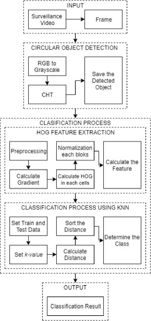
Figure 1. Proposed Method
region that is face/nose/mouth/left eye/right eye, but it can not distinguish between half and full helmet. So, they use CHT to detect the half and full helmet. Wen et al. [4]. Proposed circle arc detection based on the Circular Hough Transform method. They applied it to detect helmets through surveillance cameras at ATMs. The disadvantage of this method is that they only use the geometry feature to verify whether there is a helmet on the image captured by the camera. Geometry features are not enough to detect helmets. The head can be detected as a helmet because it is similarly circular. Rubaiyat et. al.[5]. proposed helmet detection uses for construction safety. They use Discrete Cosine Transform + Histogram of Oriented Gradient (HOG) for human detection method and Color + CHT for the helmet detection method. In this study, helmet
detection was carried out after color filtration so that helmet detection could be more accurate. However, this method will provide a disadvantage when the detected helmet is a different color. Based on the research above, we can see that CHT is good for detecting circles. Therefore it can be used to detect helmets that are also circular. Meanwhile, HOG is used to get the feature value to classify the circle that comes from the helmet itself as the main target of detection with a human head without a helmet. The classification method we chose is K-Nearest Neighbor (KNN). KNN was chosen because it is a simple method, only by setting the value for k by analyzing the number of neighbors by looking for the closest distance value as the basis for the classification parameter. Also, KNN can be applied to a multiclass system, wherein my research is divided into two classes, namely the helmet-wearing rider class and the un-helmeted rider class.
Based on the above problems and previous literature studies, we propose automatic helmet detection using Circular Hough Transform (CHT) for shape detection, Histogram of Oriented Gradient (HOG) for feature extraction, and K-Nearest Neighbor (KNN) for image classifier. Data is obtained from taking frames on surveillance videos.
In this research, the proposed method can be seen in Fig. 1. The first step is to get the image from a surveillance video. The second step is used to search for a circular object in the image using CHT. The third step is feature extraction using HOG. The fourth step is to classify the extracted feature using KNN. The last step is to get the accuracy, precision, and recall from the KNN classifier.
The video used in this research is a surveillance video that we got from a surveillance camera placed in sideroad and crossroads with a resolution of 1920x1080.
We save each frame from the video. The video has 25 fps, so we get 25 images each second of the video. After that, we save the image and will be used in the next steps.
A grayscale image or gray level image is one of the color spaces of an image. The gray level represents the number of quantization intervals in grayscale image processing. At this time, the most used method for storage is 8-bit storage. In an 8 bit grayscale image, there are 256 gray levels from 0 to 255. With 0 is black and 255 is white [6]. In this research, we used equation (1) to convert the RGB image to a grayscale image.
„ . R+G+B
Grayscale = —-— (1)
R is the intensity of the pixel in the red channel, G is the intensity of the pixel in the green channel, and B is the intensity of the pixel in the blue channel.
Circular Hough Transform (CHT) is a method to detect a circular object. Many research has been done using CHT, such as detecting a person from surveillance video[7] and cell detection for bee comb image[8]. CHT is based on the Hough transform.
To detect circle CHT is using a voting process that calculates the possibility of edge point that is lying on a circle. It uses the circle formula to set the parameter of three-dimensional space to collect votes and to search a circle within a fixed radius. The votes will be saved in an accumulator. The objective of the CHT is to find the center point from every edge point of a circle in the image through the iteration of the equation (2) and (3).
x = a + R × cos (0) (2)
y = ft + R × sin (0) (3)
Denotes a and b is the center point, R is the radius, and 0 is the angle. After the iteration accumulator with the most votes is the true center point of a circle.
Save all detected images. The stored image will later be used for training and testing data in the classification process.
-
2.3. Histogram of Oriented Gradient (HOG) Extraction

(a)

(b)
Figure 2. Aspect Ratio in HOG; (a) Original Image 69x79 pixel; (b) Resize Image 64x128 pixel
(a) (b)
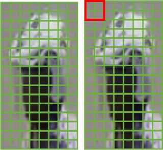
Figure 3. Two Computation Unit in HOG; (a) Cells; (b) Block
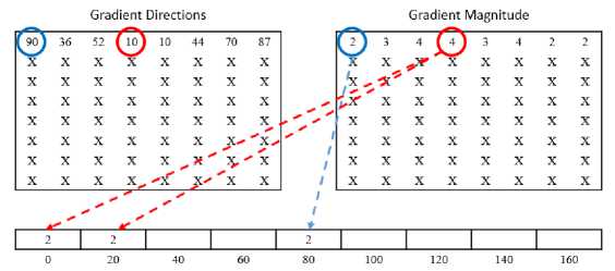
Figure 4. Calculation Process in Each Cell
Histogram of Oriented Gradients algorithm is a feature descriptor that is used to extract features from images. The algorithm is based on the distribution of the Gradient in the image. The final feature is a one-dimensional array of histograms from the extracted image. In the HOG, there are two computation units for feature extraction. It is cell and block. The cell size is 8x8 pixels, and the block size is 16x16 pixels. There are four cells in one block. Figure 3. shows the example of the two computation units for feature extraction. After the computation of the current block, it moves to the next block with an overlap of 1 cell[9].
In the preprocessing step, the HOG input image needs to have a fixed aspect ratio, so we get the same amount of feature. In this case, we use a 1:2 ratio, for example, 32x64, 64x128, or 1000x2000, but we cannot use 103x150 because it is not a 1:2 ratio. In this research, we use an image size of 64x128 pixels. Each image is scaled, keeping its aspect ratio preserve.
Therefore before we calculate the gradients, we resize every image. The example of the resize image can be seen in Figure 2.
Table 1. The Example of HOG Feature
|
Feature |
f1 |
f2 |
f3 … |
f3778 |
f3779 |
f3780 |
|
Data 1 |
0.206719 |
0.013714 |
0.077928 … |
0.054473 |
0.235448 |
0.130019 |
|
Data 2 |
0.046905 |
0.033736 |
0.033864 … |
0.019585 |
0.024376 |
0.112724 |
|
Data 3 |
0.47073 |
0.0784 |
0.006978 … |
0.000861 |
0.003578 |
0.010856 |
|
Data 4 |
0.093873 |
0.076953 |
0.025398 … |
0.043547 |
0.014677 |
0.073801 |
After we get the resized image, we calculate the Gradient. In this process, we calculate the gradient magnitude and direction from every pixel using equations (4) and (5).
g = √gX + gy (4)
θ = arctan — (5)
Bx
Denotes g is a gradient magnitude, θ is gradient direction and gx,gy is a gradient of the x-axes and y-axes. We can calculate the gx,gy by using Sobel Filtering.
in this step, we calculate the Histogram of Gradient in each cell (8x8 Pixels). The Histogram is a vector or an array of 9 bins corresponding to angles 0, 20, 40, …, 160 degrees. So we must put gradient direction and magnitude into a histogram of Gradient. The Gradient of direction is the bins or array, and the Gradient of magnitude is the value of the bins or array. The calculation process can be seen in Figure 4.
After we get the Histogram of Gradient in each cell, we normalize the Histogram from each block (16x16 pixels). A histogram normalization computation is done by combining all histograms that belong to one block. One block has four cells and has nine feature vectors, so in one block, we have 36 (4 cells x 9 bins) feature vectors. We normalize the block using equation (6).
x1n = (6)
√X2 + x∣+-+ χ326
x?is the Normalization of each block result, xl is the feature vector and i is a number feature in a block from 1 to 36.
The last step of HOG is to calculate the total feature vector from all blocks. In this research, we use an image of 64x128 pixels, so we have seven blocks in a horizontal position and 15 blocks in a vertical position. The total block we have is 105 (7x15) blocks. Each block has 36 feature vectors, so in total, we have 3780 (36x105) feature vectors. Table 1 shows an example of the HOG feature. Each data have 3780 feature vectors.
K-Nearest Neighbor algorithm [10,11] is a method for classifying objects based on the closest distance between the training data and testing data. This algorithm is a simple classifier and easy to apply an algorithm that works well with recognition issues [12]. The training process for KNN only consists of the store the features and labels from training data. The classification process only searched for distance and assigned the label from the k-nearest neighbor who has the most votes.
KNN uses a distance system to calculate classification results. Therefore it requires training data and testing data. The data is obtained from a video with a 1080p resolution and has a frame rate of 25 fps. After that, we crop the area around the head of the motorcyclist to distinguish which one belongs to the positive and negative class. Image with helmet becomes the positive class, and image without helmet becomes the negative class. The video was taken in daytime conditions, and the camera is placed on the side of a road or intersection with a height of 2-4 meters.
In this research, we used 200 data consisting of 100 helmet wearing data (positive class) and 100 non-helmet wearing data (negative class). The test data used 40 data consisting of 20 helmetwearing data (positive class) and 20 non-helmet-wearing data (negative class). The training data used 160 data consisting of 80 helmet wearing data (positive class) and 80 non-helmet wearing data (negative class).
In the KNN Classification, we need a k-value. The k-value used to determine how many calculation results will be used for voting.
In this research, we use Euclidean Distance to calculate the distance between neighbors in KNN. The equation for Euclidean distance is shown in equation (7).
dCΓr,Ty)= √tflτr - fιτyγ + (f2τr - f2τyr + - + (f3780τr - f3780τy)2 (7)
d(Tr,Ty) is the distance, Tr is testing data, and Ty is training data.
After we get the distance, we sort the distance from the smallest distance to the largest distance. Then we take some of the top data by following the k-value that has been set. For example, if we set the k-value to 5, then we take the five most top data.
The result of classification is the class that has the most votes in the k-nearest neighbor. For example, we have a k-value of 5. In the five smallest data, we have 3 data with the label of 0 and 2 data with the label of 1, so the classification result is class 0 because it has more votes than class 1 [13].
In this section, the proposed method was tested by using a dataset that we collect from several frames from the surveillance video. The output of the system is the result of the KNN classification. The result is either the circular object is the helmet-wearing class or the non-helmet wearing class.
Table 2. Sample Data of Visual Experimental Result
Actual Detected
Input
Result
1
2
3
2
1
2
2
1
(b)
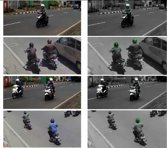
Figure 5. Example of the Dataset
The proposed method has been implemented. First, the original image is transformed to Grayscale, and CHT will be implemented to it. The CHT's purpose is to detect the head region of the motorcyclist. In this research, we select the CHT result that shows the head region because our purpose is to detect the helmet.
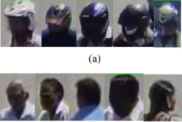
The result of CHT will be cropped and then saved to build training and testing data. The data divided into 200 training data, which was obtained from selected frames consisting of 100 helmets wearing motorcyclist head image and 100 non-helmet wearing motorcyclist head image. The test data used 40 images 20 helmet wearing motorcyclist head image and 20 non-helmet wearing motorcyclist head image that was obtained from a different surveillance video with training data. The data divided into two classes, helmet-wearing class and non-helmet wearing class. Figure 5. shows the example of the dataset.
To classify the data, we need to extract the feature from the image. We use HOG for feature extraction. There are 3780 features from each image. After that, we do labeling for each data. We do the feature extraction into both classes. The result is the same, only different in value table 2. Shows the example of the visual experimental results, the detected helmet is marked with a green circle, and the other is not marked. Several conditions cause detection failure, the image of the
head is not intact or covered with something, and the image of the head is too small. We conducted this experiment 40 times.
In order to present the performance of the proposed method, an experiment is conducted using the dataset. The measurement method uses the accuracy equation (8), precision equation (9), and recall equation (10). We use all the data in this experiment, which are 40 testing data and 160 training data. The testing data is divided by four, each has ten images, and we will calculate the average accuracy.
Table 3. Confucion Matrix
|
Predictive Relevant |
Irrelevant | |||
|
Actual |
Relevant Irrelevant |
True Positive (TP) False Positive (FP) |
False Negative (FN) True Negative (TN) | |
|
Table |
4. Testing Result | |||
|
Data |
k-value |
Accuracy |
Precision |
Recall |
|
1 |
0.80 |
0.80 |
0.80 | |
|
1 |
3 |
0.70 |
0.66 |
0.80 |
|
5 |
0.70 |
0.66 |
0.80 | |
|
7 |
0.70 |
0.66 |
0.80 | |
|
1 |
0.60 |
0.66 |
0.40 | |
|
3 |
0.60 |
0.66 |
0.40 | |
|
2 |
5 |
0.60 |
0.66 |
0.40 |
|
7 |
0.70 |
0.75 |
0.60 | |
|
1 |
1.00 |
1.00 |
1.00 | |
|
3 |
0.90 |
1.00 |
0.80 | |
|
3 |
5 |
0.90 |
1.00 |
0.80 |
|
7 |
0.90 |
1.00 |
0.80 | |
|
1 |
0.90 |
1.00 |
0.80 | |
|
3 |
1.00 |
1.00 |
1.00 | |
|
4 |
5 |
1.00 |
1.00 |
1.00 |
|
7 |
1.00 |
1.00 |
1.00 | |
|
1 |
0.825 |
0.865 |
0.75 | |
|
3 |
0.80 |
0.83 |
0.75 | |
|
Average 5 |
0.80 |
0.83 |
0.75 | |
|
7 |
0.825 |
0.852 |
0.80 | |
Table 5. Comparison Result
|
Author |
Method |
Acccuracy |
|
Wonghabut et. al. [14] |
Aspec Ratio |
74 % |
|
Rubaiyat et. al. [5] |
Color + CHT |
81 % |
|
Proposed Method |
KNN + HOG |
82.5 % |
Table 6. Computation Time Result
|
Test Number |
Time (s) |
|
1 |
1.40369 |
|
2 |
1.42919 |
|
3 |
1.48211 |
|
4 |
1.44819 |
|
5 |
1.42123 |
|
6 |
1.44429 |
|
7 |
1.43858 |
|
8 |
1.42197 |
|
9 |
1.42451 |
|
10 |
1.43190 |
|
Average |
1.43457 . _ TP+TN Accuracy = ----------- (8) j tp+tn+fp+fn v , Precision = tp (9) tp+fp v , Recall= -p- (10) tp+fn v , |
TP (True Positif) is the number of correct predictions in positive class, in this case, is the helmetwearing class, TN (True Negatif) is the number of correct predictions in negative class, in this case, is the non-helmet wearing class. FP (False Positif) is the number of incorrect predictions in the positive class, and FN (False Negatif) is the number of incorrect predictions in the negative[15]. The confusion matrix is shown in Table 3.
Testing was done by using different k-value in the KNN classifier. In this research, the k-value that users ware 1,3,5 and 7. In this research, we classify the data into two classes, the first, the helmet-wearing class, and the second, is non-helmet wearing class. Each k-value produce a different result, but the result ware satisfactory. The result of the test is shown in Table 4. The average accuracy, precision, and recall are relatively high, and it is shown that the k-value of 1 and 7 produces the highest score, but the k-value of 1 is better because it useless calculation than k-value 7. After getting the best result from our experiment, we compare it with previous research. We compare our work with two other research about helmet detection, and the result is our work produce slightly better accuracy when detecting helmet. Comparison results can be seen in Table 5.
In order to know how fast the detection time of the proposed method, we do a computation time test. The test was done on a computer that runs Microsoft Windows 10 with a processor Intel(R) Core(TM) i5-4460 and 8 GB memory. The data we use in the test is the training and testing data mention in section 2.4.1. We run the program ten times with K-value 1, and the result is shown in Table 6. The average time we got from the experiments is 1.43457 s.
In this research, we use the KNN classification because previous studies have good accuracy. Meanwhile, the consumption of computation time could be reduced by sklearn's tools in Phyton. KNN Classification uses sklearn's tools, only takes 0.4 seconds. Besides that, to increase the speed performance, we resize the original image that has a different size to become 64x128 pixel So, resizing the size of data also will be decreased the speed of KNN performance.
The test results show a computation time for each detection. This shows that the proposed method produces a fast time to detect so that it can be implemented in real-time, although the quality is poor. We can improve the quality of real-time implementation by reducing computation
time. This problem can be resolved by improving the quality of the computer or using a faster classification method.
This study comes about the detection of motorcyclists without a helmet. The system builds based on computer vision technology, which is divided as follows: shape detection, feature extraction, and image classification. The results were satisfactory.
The KNN classifier using the feature from HOG can classify between the helmet-wearing motorcyclist and the motorcyclist that is not wearing a helmet. We use different k-value in the testing process. The K-value that got the best result is 1 and 7, with an average accuracy of 82.5 % and average computation time is 1.43457 s. The present result is promising but can be improved. One of the future works is license plate recognition with the purpose of detecting the license plate from motorcyclists that are not wearing a helmet. For this, it is necessary an image with better quality to recognize the characters.
References
-
[1] Badan Pusat Statistik Kota Salatiga, “Salatiga Dalam Angka Tahun 2013,” pp. 1, 115, 155, 2013.
-
[2] L. Gicquel, P. Ordonneau, E. Blot, C. Toillon, P. Ingrand, and L. Romo, "Description of various factors contributing to traffic accidents in youth and measures proposed to alleviate recurrence," Frontiers of Psychiatry, vol. 8, no. JUN, pp. 1–10, 2017, doi:
10.11591/ijeei.v6i4.463
-
[3] P. Doungmala and K. Klubsuwan, "Half and Full Helmet Wearing Detection in Thai- land using Haar Like Feature and Circle Hough Transform on Image Processing Pathasu, " Proc. - 2016 16th IEEE Int. Conference on Computer and Information Technology CIT 2016, 2016 6th International Symposium Cloud and Service Computing IEEE SC2 2016 2016
International Symposium Security and Privacy in Social Networks and Big Data, pp. 611– 614, 2017, doi: 10.1109/CIT.2016.87
-
[4] L. J. L. C. Wen C. Chiu S., "The safety helmet detection for ATM's surveillance system via the modified Hough transform," Proceedings of Annual IEEE International Carnahan Conference on Security Technology, pp. 259–263, 2003, doi: 10.1109/CCST.2003.1297588
-
[5] A. H. M. Rubaiyat et al., "Automatic detection of helmet uses for construction safety," Proceedings - 2016 IEEE/WIC/ACM International Conference on Web Intelligence
Workshops, WIW 2016, no. November, pp. 135–142, 2017, doi: 10.1109/WIW.2016.10
-
[6] T. Kumar and K. Verma, "A Theory Based on Conversion of RGB image to Gray image," International Journal of Computer Applications., vol. 7, no. 2, pp. 5–12, 2010, doi: 10.5120/1140-1493
-
[7] H. Liu, Y. Qian, and S. Lin, "Detecting persons using hough circle transform in surveillance video," VISAPP 2010 - Proceedings of the International Conference on Computer Vision Theory and Applications, vol. 2, no. January, 2010, doi: 10.5220/0002856002670270
-
[8] L. H. Liew, B. Y. Lee, and M. Chan, "Cell detection for bee comb images using Circular hough transformation," CSSR 2010 - 2010 International Conference on Science and Social Research, no. Cssr, pp. 191–195, 2010, doi: 10.1109/CSSR.2010.5773764
-
[9] Pei-Yin Chen, Chien-Chuan Huang, Chih-Yuan Lien, and Yu-Hsien Tsai, "An Efficient Hardware Implementation of HOG Feature Extraction for Human Detection," IEEE Transactions on Intelligent Transportation Systems, vol. 15, no. 2, pp. 656–662, 2014, doi: 10.1109/TITS.2013.2284666
-
[10] K. N. Stevens, T. M. Cover, and P. E. Hart, "Nearest Neighbor Pattern Classification," vol. IT-13, no. 1, pp. 21–27, 1967.
-
[11] J. Maillo, S. Ramírez, I. Triguero, and F. Herrera, "kNN-IS: An Iterative Spark-based design of the k-Nearest Neighbors classifier for big data," Knowledge-Based System, vol. 117, pp. 3–15, 2017, doi: 10.1016/j.knosys.2016.06.012
-
[12] F. A. Mufarroha and F. Utaminingrum, "Hand Gesture Recognition using Adaptive Network Based Fuzzy Inference System and K-Nearest Neighbor," International Journal of Technology, vol. 8, no. 3, p. 559, 2017, doi: 10.14716/ijtech.v8i3.3146
-
[13] J. Kim, B.S. Kim, and S. Savarese, "Comparing Image Classification Methods: K-Nearest-Neighbor and Support-Vector-Machines," Applied Mathematics in Electrical and Computer
Engineering, pp. 133–138, 2012.
-
[14] P. Wonghabut, J. Kumphong, T. Satiennam, R. Ung-Arunyawee, and W. Leelapatra, "Automatic helmet-wearing detection for law enforcement using CCTV cameras, " IOP Conference Series: Earth and Environmental Science, vol. 143, no. 1, 2018. doi:
10.1088/1755-1315/143/1/012063
-
[15] S. Tiwari, "Blur classification using segmentation based fractal texture analysis," Indonesian Journal of Electrical Engineering and Informatics, vol. 6, no. 4, pp. 373–384, 2018. doi: 10.11591/ijeei.v6i4.463
23
Discussion and feedback