A Feature-Driven Decision Support System for Heart Disease Prediction Based on Fisher's Discriminant Ratio and Backpropagation Algorithm
on
LONTAR KOMPUTER VOL. 11, NO. 2 AUGUST 2020
DOI : 10.24843/LKJITI.2020.v11.i02.p01
Accredited B by RISTEKDIKTI Decree No. 51/E/KPT/2017
p-ISSN 2088-1541
e-ISSN 2541-5832
A Feature-Driven Decision Support System for Heart Disease Prediction Based on Fisher's Discriminant Ratio and Backpropagation Algorithm
Muh Dimas Yudianto1, Tresna Maulana Fahrudin2, Aryo Nugroho3
123 Fakultas Ilmu Komputer, Universitas Narotama
JL.Arif Rachman Hakim 51 Surabaya, Jawa Timur, Indonesia 1dimasyudianto92@gmail.com, 2tresna.maulana@narotama.ac.id, 3aryo.nugroho@narotama.ac.id
Abstract
Coronary heart disease included a group of cardiovascular, and it is a leading cause of death in low and middle-income countries. Risk factors for coronary heart disease are divided into two, namely primary and secondary risk factors. The need to identify characteristics or risk factors in heart disease patients by making the classification model. The modeling of heart disease classification to know how the system can able to reach the best prediction accuracy. Fisher's Discriminant Ratio is one of the methods for feature selection, which is used to get high discriminant features. While Backpropagation is one of the classification models to recognize patterns in heart disease patients. The experiment results showed that the accuracy of the classification model using 13 original features reached 92%. By reducing the features based on the score of the feature selection, then the lowest feature was removed from original features and left there were 12 features involved in the classification model which the accuracy increased to 93%. Furthermore, the results of determining the threshold (accuracy does not decrease continuously) and consider the effect of eliminating the lowest features that are considered quite fluctuating on accuracy. The accuracy reached 90% by eliminating the five lowest features and left eight existing features.
Keywords: Heart Disease, Discriminant Features, Fisher's Discriminant Ratio, Neural Network, Backpropagation
Coronary Heart Disease (CHD) is a heart disease that is a leading cause of death in low and middle-income countries such as Indonesia. Based on death cases caused by cardiovascular disease reached 17.1 million people per year [1]. Cardiovascular included coronary heart disease and stroke, which ranks first in chronic diseases in the world [2]. The second factor causing coronary heart disease is antioxidants [3]. Antioxidants are compounding that function to reduce the formation of free radioactive obtained from food intake. One part of antioxidants is vitamin E. The main function of vitamin E in the body is as a natural antioxidant that plays a role in capturing and inhibiting the process of lipid oxidation in the body. To inhibit oxidation, vitamin E will provide a hydrogen atom from the OH group into radical lipid peroxide, which is radical. Therefore, vitamin E is formed stable and not easily damaged and able to stop the free radical sequence with fat [4].
Hypercholesterolemia is a dangerous condition characterized by high levels of cholesterol in the blood. This is a serious problem because it is one of the main risk factors for coronary heart disease [5]. Coronary heart disease has a high mortality and illness. Although the basic cause of coronary heart disease is not known with certainty, experts have identified many factors related to the occurrence of heart disease, which is called a risk factor. The risk for coronary heart disease consists of 2 conditions, namely primary (independent) and secondary risk factors [6].
-
a. Primary risk factors: these factors can cause arterial disorders in the form of atherosclerosis
without having to be helped by other factors (independent), such as hyperlipidemia, smoking, and hypertension.
-
b. Secondary risk factors: these factors can only cause arterial abnormalities if other factors are found together, such as diabetes mellitus (DM), obesity, stress, lack of exercise, alcohol, and family history [7].
These earlier works related to heart disease research was carried out by [8] using the 13 features from [9]. All used a GA-based RFNN procedure to diagnose heart disease. The outcomes told that the percentage of accuracy rate reached 97.78%.
The other research was also carried out by [10] using data collection of Statlog Heart Disease, Cleveland heart disease, and Pima Indian Diabetes datasets from [9]. The true results of classifiers have given 93.55% and 73.77% for the Cleveland Heart Disease dataset, with two and five class labels. And 92.54% for the Pima India Diabetes dataset, also 94.44% for the Statlog Heart Disease dataset.
This research will propose the feature selection before classification using Backpropagation. The feature selection is expected to improve the quality of the dataset before classification. Various classification algorithms are widely known, such as Naïve Bayes, K-Nearest Neighbor [11], and others, but this study uses the Backpropagation algorithm, which is part of the Artificial Neural Network [12].
2. Research Methods
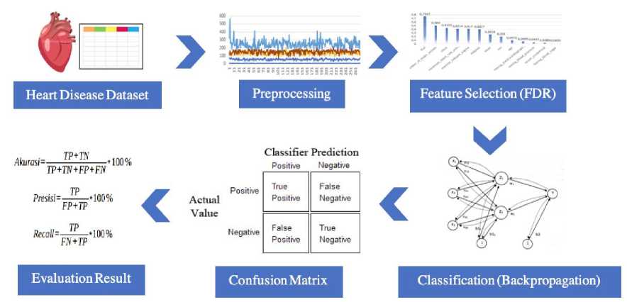
Figure 1. Proposed System Design of Heart Disease Research
The proposed system design of heart disease research is illustrated in Figure 1, begin from the collecting heart disease dataset, preprocessing dataset using Z-score normalization, selecting feature using Fisher's Discriminant Ratio, building classification model using Backpropagation and evaluating the classification model
The dataset used in this study was taken from [9] the dataset consists of heart disease status with 13 predictor features, 2 class labels, and 270 samples. We train the model using training data, which was collected from the original dataset, while the testing data was obtained from training data without labels. We want to see the accuracy of the prediction label on the testing data that match with the actual label. The features used in the heart disease dataset following Table 1.
Table 1. Heart Disease Features
|
No. |
Features |
Values |
|
1. |
Age |
Continuous {29 to 76 years} |
|
2. |
Gender |
Nominal {Male=1, Female=0} |
|
3. |
Chast |
Nominal {typical angina=1, atypical angina=2, non anginal pain=3, asymptotic= 4} |
|
4. |
Resting Blood Pressure |
Continuous in mmHg (unit) |
|
5. |
Serum Cholesterol |
Continuous in mg/dl (unit) |
|
6. |
Fasting Blood Sugar |
Nominal {>120mg/dl=1, <120mg/dl=2} |
|
7. |
Resting electrocardiographic result |
Nominal {Normal=0, Having ST-T=1, left ventricular hyperthophy=2} |
|
8. |
Maximum heart rate achieved |
Continuous in statistics |
|
9. |
Exercise-induced angina |
Nomimal {yes=1, none=0} |
|
10. |
Oldpeak |
Continuous Displaying an integer or floating value |
|
11. |
Slope |
Nominal {upsloping=1, flat=2, downsloping=3} |
|
12. |
Number of major vessels |
Continuous displaying values as integers or floats |
|
13. |
Thal |
Nominal {normal=3, fixed defect=6, reversible defect=7} |
|
14. |
Class |
Nominal {absence=0, presence=1} |
Normalization procedure with Z-score is measuring arithmetic mean values and standard deviations from existing data. If the input numbers are not distributed, the normalization of Z-scores cannot maintain the input distribution at the output. This is expected to significant facts, and the standard deviation is the optimal position and only the computation for the Gaussian distribution. For random distribution, the mean and standard deviation are fair estimates of position and measure, severally, but not optimal to drop data refinement assuring data dependences [13]. The following Z-score formula in equation (1). In our experiments, the testing data was obtained from training data that was previously used to create a model, but it is without the label. Thus, the original value of the dataset has been normalized using the Z-score. If the process is separate between training data and using testing data other than training, then the Z-score can be applied by entering testing data into the training data distribution first.
(1)
(Sy)
In the formula above, Y is the actual data for each feature, My is the average of each feature, and Sy is the standard deviation of each feature.
Fisher's Discriminant Ratio (FDR) is generally used to measure the power of discrimination of individual features in separating two classes based on their values. μ1 and μ2 each is the average value of two classes, σ1 and σ2 each is a variant of two classes in the feature to be measured. FDR is formulated as in the following equation (2).
FDR
(μi -μ)22 ( 2I+2)2)
(2)
The results given by FDR are features that have large differences in the average of the class and small variants of each class. Therefore a high FDR value will be obtained. If two features have the same absolute mean difference but differ in the number of variants of the value (σ? + σ22), then features with a smaller number of variants will get a higher FDR value. On the other hand, if two features have the same number of variants but a greater average difference, a higher FDR value will be obtained [14].
Backpropagation has numerous units that are in one or more hidden layers [15]. Figure 2 explains the Backpropagation architecture with input N (with bias), the hidden layer that happens from unit P (with bias), and the unit of output M. is the line weight from the input unit to the hidden display unit ( is the line weight connecting the bias to the input unit to hidden units). Is from the hidden layer unit to output unit Y ( is the weight of the bias in the hidden layer to the output unit ).
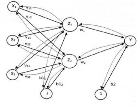
Figure 2. Backpropagation Architecture
The activation function in the Backpropagation method used in this study is the sigmoid function. The sigmoid function has values in the range of 0 to 1. Therefore, this function is used for neural networks that require output values located at intervals of 0 to 1 [16]. The sigmoid function formula follows in equation (3).
(3)
f(x) = ι+e-* with derivatives f(χ) = f(x) (1 — f(x))
While the curve of the sigmoid function is illustrated in Figure 3.
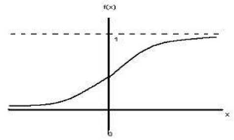
Figure 3. Sigmoid Function
The confusion matrix contains information that compares the results of the classification that should be, namely, the match between the actual label and prediction label. The following Figure 4 illustrates the confusion matrix [17].
Classifier Prediction
Actual
Value
|
Positive |
Negative | |
|
Positive |
True Positive |
False Negative |
|
Negative |
False Positive |
True Negative |
Figure 4. Confusion Matrix
The explanation of TP, TN, FN, FP as follows:
-
a. TP is True Positive, which is a match between the actual label and the predictive label on a sample of patients affected by heart disease
-
b. TN is True Negative, which is a match between the actual label and the predictive label on a sample of patients not affected by heart disease
-
c. FN is False Negative, which is a mismatch between the actual label and the predictive label on a sample of patients that are predicted to be negative (not affected by heart disease) but the facts are positive (affected by heart disease)
-
d. FP is False Positive, which is a mismatch between the actual label and the predictive label on a sample of patients that are predicted to be positive (affected by heart disease) but the facts are negative (not affected by heart disease)
The evaluation result is an assessment using a formula by comparing the portion of data that is correctly classified and the portion of data that is misclassified [18]. Table 2 showed the evaluation result using accuracy, precision, and recall.
Table 2. Evaluation Result
|
Evaluation |
Formula |
|
Accuracy |
TP + TN ∗ 100% TP + TN + FP + FN TP |
|
Precision |
∗ 100% FP + TP TP |
|
Recall |
∗ 100% FN + TP |
The explanation of accuracy, precision, and recall as follows:
-
a. Accuracy is the percentage of comparison between correctly classified data and the whole data.
-
b. Precision is the percentage of the amount of confident category data (heart disease) that is precisely classified divided by the total data classified as positive.
-
c. Recall is the percentage of the amount of confident category data (heart disease) accurately classified by the system.
The experiment result of this research reported about the normalization of data distribution, feature selection using Fisher's Discriminant Ratio, which was represented in feature ranking, classification for building model using Backpropagation, and also evaluation using confusion matrix.
3.1 Preprocessing using Z-score normalization
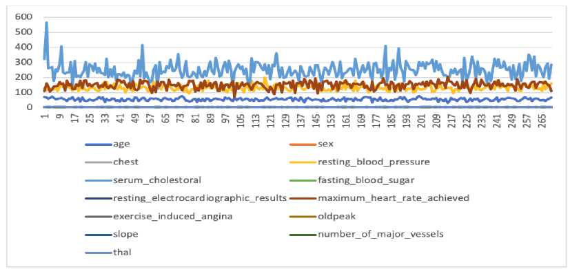
Figure 5. The Data Distribution Before Normalization
Figure 5 illustrates the condition of the original data of heart disease before the normalization process. The range or scale of data for each feature varies, feature values are mixed between units, tens, and hundreds. This results in the dimensions of the dataset being unbalanced. The X-axis represents the data sequence number, the Y-axis is the data value, and the colored lines show different features, whereas the results of normalization using the Z-score are illustrated in Figure 6.
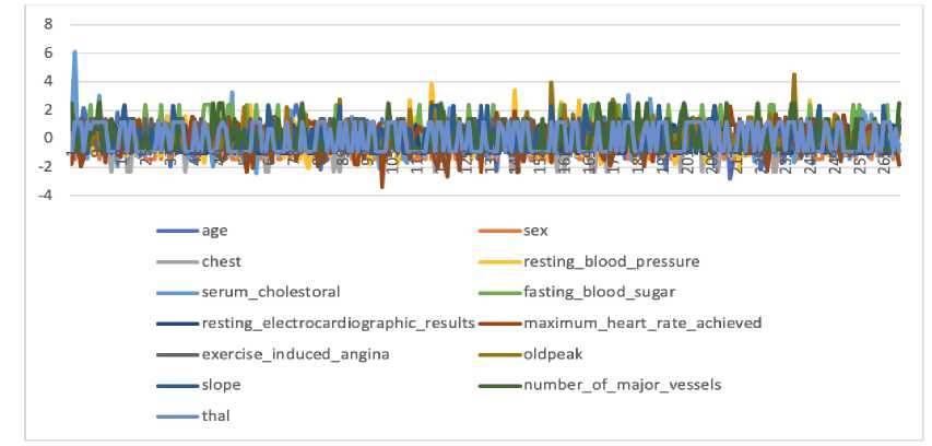
Figure 6. The Data Distribution After Normalization
Figure 6 illustrates the normalized heart disease data distribution, where the data scale for each feature is on a balanced scale, it is between -3 to 3. The X-axis represents the data sequence number, the Y-axis is the Z-score value, and the colored lines show different features.
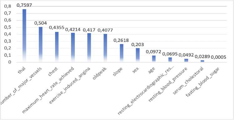
Figure 7. Feature Selection using Fisher's Discriminant Ratio
The feature selection process will test each of the features, which is the most influential features of the dataset. At the beginning process, Fisher's Discriminant Ratio (FDR) splits the dataset into two groups according to their class. Second, it calculates the average of each feature in its own class. Third, it calculates the total variance of each feature in its own class. Fourth, it calculates the FDR value using equation (2) from the second and third calculation results. The X-axis shows the names of the predictor features, while the Y-axis is the FDR score for each predictor feature.
Figure 7 was illustrated the feature selection, which was represented in Feature Ranking by FDR. In the test results, it was reported that the 'thal' feature has a high discriminant value on the dataset reached 0.75976, while 'fasting blood sugar' feature has a low discriminant value only reached of 0.000541.
The backpropagation method of this research used 13 features with two classes. Backpropagation architecture in this experiment consists of 13 input neurons (13 features) and one output neuron (two classes: 0 or 1). The number of hidden layers in this experiment used one hidden layer with four neurons. To determine the number of neurons in the hidden layer, used the formula √ (m x n), where m is the input layer, and n is the output layer. Therefore, the number of neurons in the hidden layer are obtained optimally. The tools used in this experiment are Python programming language, we configure the Backpropagation with the number of learning rates = 30, target error = 0.5.
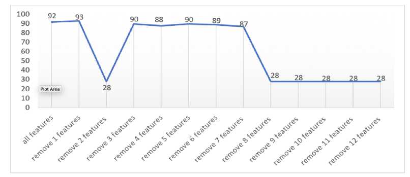
Figure 8. The Effect of Feature Selection on The Accuracy Classification
Figure 8 illustrated the classification result when all features involved in the classification model reached 92%, and the next step was carried out to remove the first lowest feature with an accuracy value reached 93%. Then, it was removed the two lowest features with an accuracy reached 28%, and the accuracy was increased to reach 90% when removed the three lowest features. It was continued to remove the four lowest features with an accuracy that decreased to 88%, and the accuracy was increased to reach 90% when removed five lowest features. The eight features obtained are the features that have the best discrimination level, while the five eliminated features do not mean anything to the dataset because the level of discrimination is low. When it was removed the six lowest features, the accuracy was decreased to 89% and getting decreased until it removed the 12 lowest features, in which the accuracy reached 28%.
The feature selection process as a way to determine whether the effect of accuracy is generated when built classification model by reducing the lowest number of features through feature selection by the FDR. We analyze the results of this experiment to show that when removing the two lowest features, accuracy reaches 28%. This indicates that the second-lowest feature (serum cholesterol) is an important feature, while the first lowest feature is not important (fasting blood sugar). Then, the model chosen is the dataset that has eliminated the first lowest feature (fasting blood sugar) that can achieve 93% accuracy. Therefore, it remains decided that the highest-level accuracy in the classification model of the heart disease dataset was reached 93% by removing one feature. However, to determine the number of features that need to be removed from the dataset does not depend on increasing accuracy at the beginning of removing the lowest features, but also looking at fluctuations or accuracy that occur when a number of features are removed.
To know the performance of the classification model based on the Backpropagation algorithm, it needs to use the confusion matrix. This matrix helped to know the frequency of match between the actual label and predicted label.
Table 3. Confusion Matrix Result of Heart Disease (Original Features)
|
Presence |
Absence | |
|
Presence |
143 |
7 |
|
Absence |
15 |
105 |
Table 4. Classification Accuracy Result of Heart Disease (Original Features) Target Precision Recall Accuracy
0 0.91 0.95
1 0.94 0.88 0.92
Table 3 reported that there are 143 heart disease patients who match between the actual label: presence and predicted label: presence (True Positive), while seven patients who are no match between the actual label: presence and predicted label: absence (False Negative). The other cases reported there are 105 heart disease patients who match between the actual label: absence and predicted label: absence (True Negative), while 15 patients who are no match between the actual label: absence and predicted label: absence (False Positive). Therefore, the evaluation results in Table 4 reported that the precision of target 0: 91% and recall 95%, while the precision of target 1: 94% and recall 88%. Then, the accuracy of the classification reached 92%. Table 3 and Table 4 are reported of the experiment using 13 original features of heart disease.
In the second dataset by using Fisher Discriminant Ratio (FDR) results which was removed the first lowest feature scores, the test results obtained are:
|
Table 5. Confusion Matrix Result of Heart Disease (FDR Features) | ||
|
Presence |
Absence | |
|
Presence |
142 |
8 |
|
Absence |
10 |
110 |
Table 6. Classification Accuracy Result of Heart Disease (FDR Features)
|
Target |
Precision |
Recall |
Accuracy |
|
0 |
0.93 |
0.95 | |
|
1 |
0.93 |
0.92 |
0.93 |
Table 5 reported that there are 142 heart disease patients who match between the actual label: presence and predicted label: presence (True Positive), while eight patients who are no match between the actual label: presence and predicted label: absence (False Negative). The other cases reported there are 110 heart disease patients who match between the actual label: absence and predicted label: absence (True Negative), while ten patients who are no match between the actual label: absence and predicted label: absence (False Positive). Therefore, the evaluation results in Table 6 reported that the precision of target 0: 93% and recall 95%, while the precision of target 1: 93% and recall 92%. Then, the accuracy of the classification reached 93%. Table 5 and Table 6 are reported of the experiment using 12 features of heart disease based on FDR scores. %. The results of the accuracy level in this study are similar to the research of [10] with an accuracy rate of CHD 93.55%. But must get the same results, this study provides another contribution in the form of feature selection from 13 existing features become smaller. There is also a study with the same result, which is 93.33% using the χ2-Gaussian Naive Bayes method [19].
The classification of heart disease using the Fisher Discriminant Ratio (FDR) and Backpropagation obtained pretty good results. Feature selection using FDR applied to 13 features that had been carried out the normalization process with the Z-score before, it was
given results that 'thal' feature as the highest discriminant feature with a score of 0.75976 while 'fasting blood sugar' feature as the lowest feature with a score of 0.000541. The classification model using Backpropagation reached an accuracy to 92% with 13 original features of the heart disease dataset. The feature selection using Fisher's Discriminant Ratio was given the important information that there is the one lowest discriminant feature with the lowest score of the heart disease dataset, which recommended removing from the dataset. Therefore, the combination between FDR and Backpropagation, given the improvement of classification model accuracy of heart disease dataset, reached 93. The suggestion for future works is needed to evaluate the feature not only single feature evaluation like Fisher's Discriminant Ratio, but also use multi-features evaluation like exhaustive search algorithm to obtain the best combination feature and can improve the accuracy of the classification model.
References
-
[1] L. DeRoo et al., "Placental abruption and long-term maternal cardiovascular disease mortality: a population-based registry study in Norway and Sweden," European Journal of Epidemiology, vol. 31, no. 5, pp. 501–511, 2016.
-
[2] L. Soares-Miranda, D. S. Siscovick, B. M. Psaty, W. Longstreth Jr, and D.
Mozaffarian, "Physical activity and risk of coronary heart disease and stroke in older adults: the cardiovascular health study," Circulation, vol. 133, no. 2, pp. 147–155, 2016.
-
[3] P. Zhang, X. Xu, X. Li, and others, "Cardiovascular diseases: oxidative damage
and antioxidant protection," European Review for Medical and Pharmacological Sciences, vol. 18, no. 20, pp. 3091–3096, 2014.
-
[4] K. A. Wojtunik-Kulesza, A. Oniszczuk, T. Oniszczuk, and M. Waksmundzka-Hajnos, “The influence of common free radicals and antioxidants on development of Alzheimer’s Disease,” Biomedicine & Pharmacotherapy, vol. 78, pp. 39–49, 2016.
-
[5] U. Bhalani and P. Tirgar, "A Comparative Study for Investigation into Beneficial Effects of Ketoconazole and Ketoconazole+ Cholestyramine Combination in Hyperlipidemia and The Complications Associated With It.," Advances in Bioresearch, vol. 6, no. 4, 2015.
-
[6] J. L. Mega et al., "Genetic risk, coronary heart disease events, and the clinical benefit of statin therapy: an analysis of primary and secondary prevention trials," The Lancet, vol. 385, no. 9984, pp. 2264–2271, 2015.
-
[7] J. Bruthans et al., "Educational level and risk profile and risk control in patients with coronary heart disease," European Journal of Preventive Cardiology, vol. 23, no. 8, pp. 881–890, 2016.
-
[8] K. Uyar and A. Ihan, "Diagnosis of heart disease using genetic algorithm based trained recurrent fuzzy neural networks," Procedia Computer Science, vol. 120, pp. 588–593, 2017.
-
[9] "UCI Machine Learning Repository: Heart Disease Data Set."
https://archive.ics.uci.edu/ml/datasets/Heart+Disease (accessed May 02, 2020).
-
[10] K. B. Nahato, K. H. Nehemiah, and A. Kannan, "Hybrid approach using fuzzy sets and extreme learning machine for classifying clinical datasets," Informatics in Medicine Unlocked, vol. 2, pp. 1–11, 2016.
-
[11] A. R. Pratama, M. Mustajib, and A. Nugroho, “Deteksi Citra Uang Kertas dengan Fitur RGB Menggunakan K-Nearest Neighbor,” Jurnal Eksplora Informatika, vol. 9, no. 2, pp. 163–172, Mar. 2020, doi: 10.30864/eksplora.v9i2.336.
-
[12] Mirwan, A. Nugroho, F. Hendarta, R. Hidayatillah, F. Hassan, and K. P. Nana, "Virtual Assistant Using Lstm Networks In Indonesian," in 2018 International Seminar on Research of Information Technology and Intelligent Systems (ISRITI), Nov. 2018, pp. 652–655, doi: 10.1109/ISRITI.2018.8864448.
-
[13] S. Jain, S. Shukla, and R. Wadhvani, "Dynamic selection of normalization techniques using data complexity measures," Expert Systems with Applications, vol. 106, pp. 252–262, Sep. 2018, doi: 10.1016/j.eswa.2018.04.008.
-
[14] M. F. Tresna, S. Iwan, and R. B. Ali, "Data Mining Approach for Breast Cancer Patient Recovery," EMITTER International Journal of Engineering Technology, vol. 5, no. 1, pp. 36–71, 2017.
-
[15] N. Borisagar, D. Barad, and P. Raval, "Chronic Kidney Disease Prediction Using Back Propagation Neural Network Algorithm," in Proceedings of International Conference on Communication and Networks, 2017, pp. 295–303.
-
[16] A. Wanto, A. P. Windarto, D. Hartama, and I. Parlina, "Use of Binary Sigmoid Function And Linear Identity In Artificial Neural Networks For Forecasting Population Density," International Journal of Information System and Technology, vol. 1, no. 1, pp. 43–54, 2017.
-
[17] B. M. Jadav and V. B. Vaghela, "Sentiment analysis using support vector machine based on feature selection and semantic analysis," International Journal of Computer Applications, vol. 146, no. 13, 2016.
-
[18] Z. Cömert and A.F Kocamaz, "Comparison of machine learning techniques for fetal heart rate classification," Acta Physica Polonica A, vol. 132, no. 3, pp. 451– 454, 2017.
-
[19] L. Ali et al., "A Feature-Driven Decision Support System for Heart Failure Prediction Based on χ2 Statistical Model and Gaussian Naive Bayes," Computational and Mathematical Methods in Medicine, 2019, doi:
10.1155/2019/6314328.
75
Discussion and feedback