EFFECTIVE BANDWIDTH FOR SELF-SIMILAR TRAFFIC IN ATM NETWORK
on
Effective Bandwidth for …
Linawati, Sri Ariyani
EFFECTIVE BANDWIDTH FOR SELF-SIMILAR TRAFFIC IN ATM NETWORK
Linawati, Ni Wayan Sri Ariyani Electrical Engineering Department Udayana University, Jimbaran, Bali, Indonesia
ABSTRACT
This paper proposes a new approach to estimate the effective bandwidth for self-similar traffic in ATM network. In this approach we use the tail distribution of queue length based on FBM model. This approach is derived from the inequalities for Mills’ ratio. Then a comparison with Norros and Trinh&Miki schemes are analysed. The results demonstrate reasonable agreement between numerical and simulation results and between all schemes. Their bandwidth estimation tends closer for CLP improvement.
Key Words: effective bandwidth, CLP, FBM, self-similar traffic, ATM
Effective bandwidth is a measurement of a traffic stream in modern communication networks. One of the characteristics of these networks is that many connections are multiplexed, or aggregated, over a common cable. The issue then is to determine the number of connections that can be multiplexed without violating any service levels guaranteed to the customers. If the connection is based solely on its peak rate, then clearly there will be wasted bandwidth on the cable, as the connection will likely not send bytes at the peak rate continuously. On the other hand, if it based on the mean rate, that there may be times where the connection cannot provide the service to the incoming traffic stream, as it will occasionally send bytes at its peak rate. Thus, a decision has to be made based on some parameters lying between the mean and peak rate. Effective bandwidth allows us to do this, as it is a compromise between these two extremes number.
Several approach for determining effective bandwidths have been derived for short-range dependence (SRD) and long-range dependence (LRD) [1, 2, 3, 4]. The notion of effective bandwidth itself is a measurement of the resource requirements of a traffic stream with certain quality of service (QoS) constraint. The effective bandwidth depends sensitively on the source statistical properties as well as system parameters, e.g., buffer size, service discipline.
In this paper, a new approach is proposed to derive an effective bandwidth for self-similar traffic, which is based on Fractional Brownian Motion (FBM) model. This approach is derived from the inequalities for Mills’ ratio [6]. Then a comparison with previous schemes and simulation result is presented here.
In section 2, an overview of some effective bandwidth schemes is presented. Then a new approach of effective bandwidth for self-similar traffic is proposed here. The numerical and
simulation results with a discussion of the schemes comparisons using the FBM traffic model as a common basis are shown in section 3. Finally conclusions are presented in section 4.
A self-similar traffic that adopts FBM as its model can be described as [1]:
A(t) = mt + sqrt(am) Zt (1)
Where m is mean rate, a is variance coefficient and Zt is the increment of FBM.
For determining the effective bandwidth of this traffic model, Norros [1] approximates the tail behaviour of queue length distribution as a Weibull distribution. From the lower bound of CLP (cell loss probability) (2), the effective bandwidth (C) can be derived for buffer size (B) (3).
θ2
≈ exp(-(C^Lb2-2H) 2k(H)2am
(2)
C = m + (k(H)√-2lnε)H a(2H)B“(1“H)/Hm(2H)(3)
with k(H) = Hh (1 - H)1 h , H =Hurst parameter, and
am tH
Another scheme is proposed by Trinh and Miki [2]. They approximate buffer queue as a Weibull distribution as well in order to derive the bandwidth allocation. By using approximation in (4) the bandwidth allocation can be defined in (5). However slight modification has been done in this
effective bandwidth by eliminating the prediction factor since the traffic predictor is not employed here.
2
(-2lnε-4) 0.5σ HH(1-H)1-H
B1-H
(5)
Where σ is standard deviation.
This scheme is based on cell loss probability too and valid for large queue length tail asymptotic of large buffer size.
As stated in [5], the CLP can be defined as:
∞2
ε=P[X >B]= ∫exp(-X ) dx=1-N(θ)(6)
2πθ 2
Then the tail distribution can be approximated by the inequalities for Mills’ ratio [6]. These inequalities can be interpreted as bounds for N(θ).
21
12[1+(1-exp(-θ2 )2]≤N(θ)
1 N(θ)≤ 12[1+(1-exp(-θ2)2]
(7)
Then the lower bound of CLP (ε) can be defined as:
The maximum value of θ occurs at
* t
HB
(1 - H)(C - m)
then
1
-
θ* = (am) 2(C-m)H(B)1-H(1-H)H-1(H)-H(9)
Therefore the lower bound of effective bandwidth can be estimated as:
C=m+(-2ln(y)am) 2H(B) H (1-H) H (H)
Where: y=1-(1-2ε)2 .
Comparisons between numerical and simulation results are discussed in this section. The simulation model that is implemented here is based on discrete time advance algorithm (DTA) [5]. The
general algorithm is expressed as a simulation program in the following pseudocode:
while i < time limit,
% new arrivals
-
arrival = load pOCT89;
-
no_cell = queue_cell + arrival;
% serve the cells (service rate) if no_cell > 0 then
no_cell = no_cell – service_rate;
else
no_cell = 0;
-
% Store the cells that are not served yet if no_cell >= buffer_capacity
-
cell_loss = no_cell – buffer_capacity;
-
buffer = buffer_capacity;
else
-
buffer = no_cell;
-
queue_cell = buffer;
end
% advance time to next time slot
i = i + 1;
end
In this simulation, the CLP is not an input parameter in the simulation configuration. It is, relatively, an output result of the simulation. As traffic input, a capture traffic trace from Bellcore Ethernet traffic data pOct89 is selected [7]. Only 1024 seconds of traffic has been employed in this simulation process. The Hurst parameter, mean and coefficient of variance of this traffic are H=0.78, m=2279 kbps, a=262.8 kbits.sec. Buffer size (B), Hurst parameter (H), and bandwidth (C) are set as follows, B is varied between 100 kbits up to 2000 kbits, H-parameter from 0.5 to 0.9, and from 3000 kbps up to 4500 kbps for bandwidth allocation (C).
-
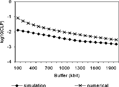
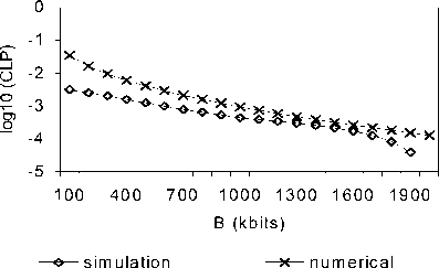
Figure 1 presents a comparison between numerical and simulation results of cell loss probability at various buffer sizes and various bandwidths. It describes precisely the relationship between buffer size and CLP for H at 0.78 and C from 3000 up to 4500 kbps (not to be seen here, due to space limitation). Generally, numerical results and simulation results agree well here. The increasing of buffer size cannot decrease the CLP dramatically, except it is shown in simulation results for C=4 Mbps and B>1700 kbits, the CLP drops sharply for slight increases of buffer. On the other hand, the increasing of bandwidth shows significant decreasing of CLP respectively, in particular in the simulation result; CLP is going down sharply for large bandwidth (C=4500 kbps) and buffer size (B>600 kbits) (see Figure 2).
-
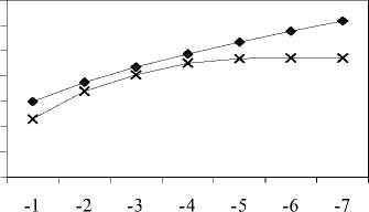
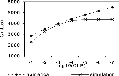
Figure 2 plots the comparison between numerical and simulation results for effective bandwidth estimation. The bandwidth estimation has done for different size of buffer, H=0.78, CLP from 10-1 down to 10-7. Surprisingly, it shows that the
simulation result tends to be steady for CLP less than 10-4. As a consequence, a gap between simulation results and numerical results become wider when CLP reaches less than 10-4. Simulation results imply at a certain level of bandwidth capacity for fixed buffer size, the CLP will decrease sharply for slight increase of bandwidth.
(a) C=3500 kbps
(b) C=4000 kbps
Figure 1. CLP for various Buffer sizes (H=0.78)
7000
6000
5000
⅛ 4000
r 3000
2000
1000 0
—♦— numerical simulation
log10(CLP)
-
(a) B=500 kbits
-
(b) B=1000 kbits
-
Figure 2. Effective Bandwidth for various CLP
Figure 3 emphasizes that by enlarging buffer size from 500 kbits to 2000 kbits, does not improve the performance of system in term of CLP for high degree of self-similar traffic. For lower H-parameter (H<0.8), the increasing of buffer size reduces the need of bandwidth capacity, for example when B increases from 500 kbits up to 2000 kbits, then C decreases from 6500 kbps down to 3800 kbps (H=0.6). As a result for high degree self-similar traffic, it does not need big size of buffer, instead of no improvement in CLP, it causes bigger delay in network system.
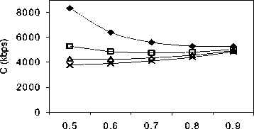
H-parameter
♦ B=500 B=1000
B=1500 B=2000
-
Figure 3. H-parameter vs. Bandwidth Estimation (C)
Figure 4 compares the proposed approach with Norros and Trinh&Miki approaches for CLP and bandwidth estimation. Their numerical results agree well. Norros approach estimates CLP and bandwidth above others. For example Norros approach is one order of magnitude over the proposed approach and approximately one and half order of magnitude over Trinh&Miki approach for CLP estimation. On the other hand, the proposed approach is between the two approaches for CLP and bandwidth prediction.
Notice in Figure 4b, the gap between all schemes tends narrower when the CLP declines, therefore they
have close bandwidth estimation, for example, for CLP=10-6, Norros approximates C=5353 kbps, Trinh&Miki approximates C=5146 kbps and proposed scheme approximates C=5151 kbps.
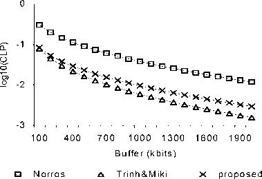
(a) CLP Estimation
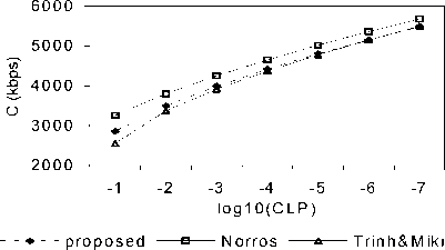
(b) Bandwidth Estimation
-
Figure 4. Comparisons between all approaches
These observations conclude that the proposed approach can predict CLP and bandwidth estimation for self-similar traffic based on FBM model. This
approach agrees well with Norros and Trinh&Miki approaches and its bandwidth estimation is between both schemes.
Since the large buffer size does not increase the performance of system for high degree of self-similar traffic, it is still a challenging area to estimate the right buffer allocation to achieve better CLP and delay of system when the input is a self-similar traffic.
REFERENCES
-
[1] Norros I., On the Use of Fractional Brownian Motion in the Theory of Connectionless Networks, IEEE J. on selected areas in comm., vol. 13, no.6, August 1995, 953-962.
-
[2] N.C. Trinh and T. Miki, Dynamic Resource Allocation for Self-Similar Traffic in ATM Network, IEEE, 5th APCC/OECC, 1999, Vol. 1, pp. 160-165.
-
[3] S.K. Biswas and R. Izmailov, Design of a Fair Bandwidth Allocation Policy for VBR Traffic in ATM Networks, IEEE/ACM Trans. On Networking, Vol. 8, No. 2, April 2000, pp. 212223.
-
[4] A.W. Berger and Y.Kogan, Dimensioning Bandwidth for Elastic Traffic in High-Speed Data Networks, IEEE/ACM Trans. On Networking, Vol. 8, No. 5, October 2000, pp. 643-654.
-
[5] Linawati and H. Mehpour, Cell Loss Analysis of Self-Similar Traffic in ATM Network, IEEE APCCAS, December 2002, Singapore.
-
[6] N.I. Johnson and S. Kotz, Continuous Univariate Distributions-1, John Wiley & Sons, USA, 1970.
-
[7] Will Leland and Dan Wilson, Bellcore Morristown Research and Engineering, http://ita.ee.lbl.gov/html/traces.html.
Teknologi elektro
4
Vol.3 No. 2 Juli – Desember 2004
Discussion and feedback