Implementation Learning Vector Quantization(LVQ) for Chronic Kidney Disease Classification
on
p-ISSN: 2301-5373
e-ISSN: 2654-5101
Jurnal Elektronik Ilmu Komputer Udayana
Volume 9 No. 2, November 2020
Implementation Learning Vector Quantization (LVQ) for Chronic Kidney Disease Classification
I Gst Bgs Bayu Adi Pramanaa1, I Made Widiarthaa2, Luh Gede Astutia3
aInformatics Department, Udayana University
Bali, Indonesia
Abstract
Chronic kidney disease is a disruption in the function of the kidney organs. When the kidneys are no longer fully functioning, the body is filled with water and a waste product called uremia. As a result, the body or legs will experience swelling and feel tired quickly because the body needs clean blood. Therefore, impaired kidney function should not be underestimated because it can be fatal. Researchers have conducted research related to the classification of kidney disease to find out what symptoms can cause kidney disease. One method that can be used for classification is the Learning Vector Quantization (LVQ) method. In this study, the LVQ algorithm was applied to classify chronic kidney disease. From the research results, the highest accuracy is 81.667% with the optimal learning rate is 0.002.
Keywords: Kidney Disease, Learning Vector Quantization, Classification, Euclidean, Dataset
Chronic kidney disease is a clinical syndrome, in which the disease is caused by a chronic, progressive, persistent, and irreversible decline in kidney function [1]. When the kidneys are no longer fully functioning, the body is filled with water and a waste product called uremia. As a result, the body or legs will experience swelling and feel tired quickly because the body needs clean blood. Therefore, this chronic kidney disease should not be underestimated because it can be fatal.
Researchers have conducted various studies on the classification of chronic kidney disease. In 2019, Ardina Ariani conducted a researched classification of kidney disease using K-Nearest Neighbor. The results of the research conducted got an accuracy of 85, 83% [2]. Apart from using the KNN method, another method that can be used for classification is the Learning Vector Quantization method. LVQ is a method of classifying patterns for each existing unit with an output that will represent a certain class or predetermined category [3]. In 2016, Rudi Hariyanto researched the classification of cataract eye diseases based on pathological disorders with the Learning Vector Quantization algorithm. The results of the calculation analysis using the LVQ method produce an accuracy of 98% with a computation time of 0.01 seconds [4]. The next research using the LVQ method was carried out in 2019 by Romlah Tantiati, wherein his research using the LVQ method for labor classification. The accuracy results obtained in this study amounted to 93, 78% [5].
Based on several studies that have been described, it appears that the Learning Vector Quantization method produces better accuracy results than the KNN method in classification problems. In this study will research the implementation of the Learning Vector Quantization Method for the Classification of Chronic Kidney Disease. The data used in this study is chronic kidney disease data sourced from the Kaggle database
https://www.kaggle.com/mansoordaku/ckdisease.
In this study, the classification process will be carried out at the data processing stage. The data that has been collected will be carried out by a preprocessing process first, normalization process used to made the data does not have a very far range of values for each feature, the next preprocessing stage is to divide the data into 2 parts, namely training data and testing data. After the data is ready, data processing will be carried out using the Learning Vector Quantization method to produce a classification of chronic kidney disease. An overview of the research methodology can be seen in Figure 1:
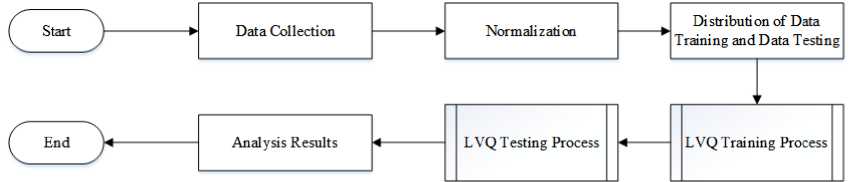
Figure 1. Research Method Flowchart
In this study, the data used were secondary data obtained from the data bank https://www.kaggle.com/mansoordaku/ckdisease, namely a dataset of chronic kidney disease. In the dataset, there are 400 data records that have 24 features and 1 output in the form of classification results for chronic kidney disease and not chronic kidney disease. In the dataset of chronic kidney disease, there is a missing value, so a preprocessing stage will be carried out to overcome the missing data. The description of each feature dataset based on the data domain can be seen in Table 1:
Table 1. Domain Dataset Feature
|
Feature |
Domain |
|
Age |
2 -90 |
|
Blood Pressure |
50 - 180 |
|
Specific Gravity |
1,005 – 1,025 |
|
Albumin |
0 - 5 |
|
Sugar |
0 – 5 |
|
Red Blood Cell |
Normal/Abnormal |
|
Pus Cell |
Normal/Abnormal |
|
Pus Cell Clumps |
Present/NotPresent |
|
Bacteria |
Present/NotPresent |
|
Blood Glucose Random |
22 - 490 |
|
Blood Urea |
1,5 – 391 |
|
Serum Creatinine |
0,4 – 76 |
|
Sodium |
4,5 – 163 |
|
Pottasium |
2,5 - 47 |
|
Hemoglobin |
3,1 - 17,8 |
|
Packed Cell Volume |
9 - 54 |
|
White Blood Cell Count |
2200-26400 |
|
Red Blood Cell Count |
2,1 - 8 |
|
Hypertension |
Yes/No |
|
Diabetes Mellitus |
Yes/No |
|
Coronary Artery Disease |
Yes/No |
|
Appetite |
Good/Poor |
|
Pedal Edema |
Yes/No |
|
Ane |
Yes/No |
|
Class |
Ckd/Nockd |
2.2 Normalization Data
Before normalizing, data that has missing values will be carried out at the preprocessing stage first by entering data using a substitution technique with the mean calculation technique for numeric data and mode for categorical data. At this stage, it will also replace word-type data to numeric [2]. After the data is ready, the normalization stage will be carried out. Data normalization aims to equalize the domain value of each feature in the dataset. In this study, using MinMax Scalar Normalization can be done with an equation 1 [2]:
x-Dmin
y =
Dmin-Dmax
(1)
Where: y
x
= result of normalization
= the data value to be normalized
Dmax = the maximum value of data to be normalized
Dmin = the minimum value of data to be normalized
The dataset will be normalized using formula (1). The data normalization process carried out using Microsoft Excel tools.
The distribution of training data and testing data uses a ratio of 7:3, which is 70% for training data and 30% for testing data.
In data processing, the Learning Vector Quantization(LVQ) method will be implemented with the scenario that is to change the learning rate value to get a good accuracy value. LVQ has two processes when doing classification, including the training process and the testing process. Process training will produce a weight vector that will be the reference for the testing process, optimal weight vector is needed to produce classification results that have high accuracy.
-
2.4.1 LVQ Training Process
FL OWCHART FOR TRAINING LVQ
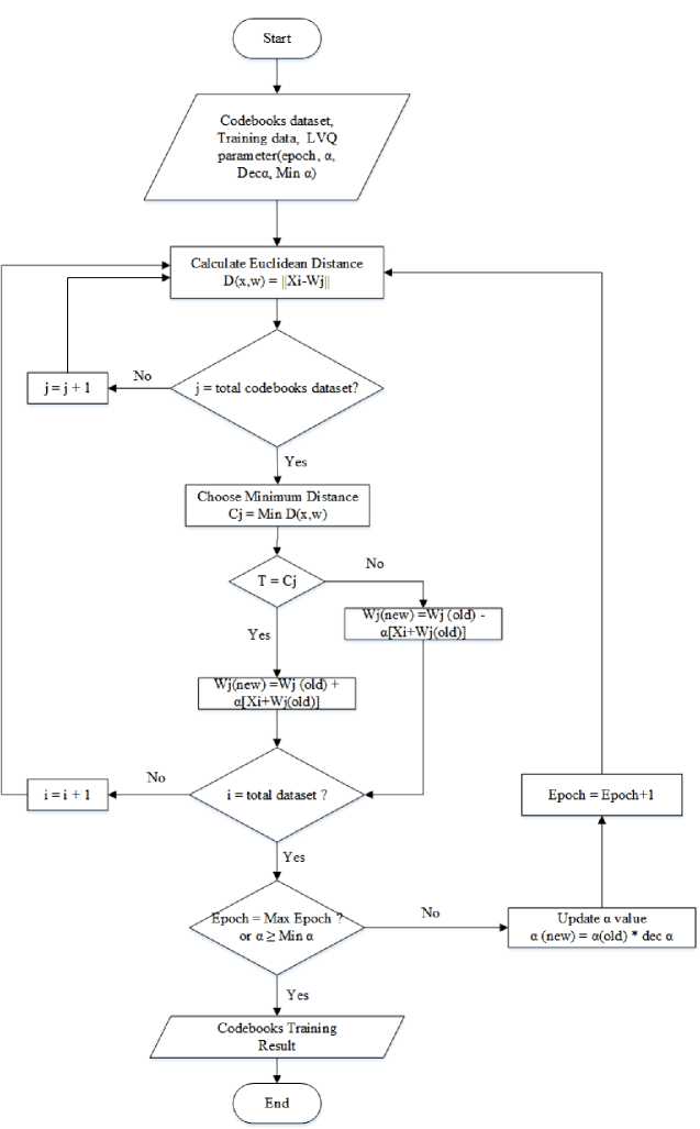
Figure 2. Flowchart LVQ Training
The following is an explanation of the Figure 2 LVQ Training Flowchart [6]:
-
1. In this LVQ training, we will train the codebooks of the LVQ vector which will be used in the LVQ testing stage. The first stage in this training is to determine the value of α (learning rate), dec α (reducing the learning rate), min α (minimal learning rate), training data, and epoch.
-
2. Perform euclidean weight calculations using the formula (2).
D(x,w) = ^Xl-Wj Il (2).
-
3. Determine the minimum distance using the formula (3).
Cj = Miri D(x,w) (3).
-
4. Make a comparison between the minimum distance (Cj) and the target (T). If the minimum distance (Cj) is equal to the target value (T), then the weight will be updated using the formula (4):
Wj (new) = Wj (old) + a[Xi - Wj(old)](4).
Meanwhile, if the minimum distance (Cj) is not the same as the target (T), then the weight will be updated using the formula (5):
Wj(new) = Wj(old)- a[Xi- Wj(old)](5).
-
5. Repeat the second to fourth process as much as the existing training data.
-
6. Update the α value using the formula (6):
-
7. Repeat the second to sixth poses until the maximum iteration or learning rate α has been maximum.
-
8. The weight of LVQ training has been obtained and will be used in the LVQ testing.
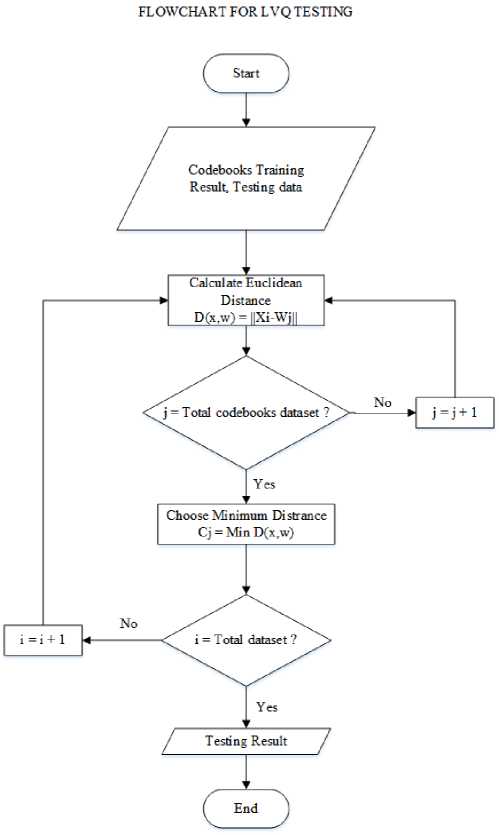
Figure 3. Flowchart LVQ Testing
The following is an explanation of the Figure 3 LVQ Testing Flowchart [6]:
-
1. The LVQ testing stage is the stage for determining the results of the classification using the weight vector of the LVQ training results. The first stage in this training is to use the codebooks of the LVQ training results as initial weights and enter the testing data.
-
2. Perform euclidean weight calculations using the Euclidean formula (2).
-
3. Determine the minimum distance using formula (3).
-
4. If the target value of the minimum values is equal to one, it is classified as a person with chronic kidney disease. Meanwhile, if the target value of the minimum values is equal to zero, it is classified as not having kidney disease.
-
5. Repeat the second to fifth process as much as the available training data.
-
6. The classification results have been obtained.
In this study, the accuracy of the classification of kidney disease using the LVQ method analyzes, wherein the testing process, the parameters changed is the learning rate from 0.001, 0.002, 0.003, 0.004, 0.005, 0.006, 0.007, 0.008, 0.009 as many as 25 iterations, dec α (deducting learning rate) with a value of 0.4 and min α (minimum learning rate) with a value of 0.0000001.
At the data processing stage, it will be implemented using the PHP programming language. In its implementation, testing and training data is used, the ratio used is 7:3. If it is used as a percentage of 70% for Training data, and 30% for Testing data. In this study, the number of features used is in accordance with the data that has been described in the data collection process. Experiments for parameters were carried out by changing the learning rate to 0.001, 0.002, 0.003, 0.004, 0.005, 0.006, 0.007, 0.008, 0.009 of 25 iterations, dec α (reducing learning rate) with a value of 0.4 and min α (minimum learning rate) with a value 0.0000001. The accuracy results can be seen in Table 2:
Table 2. Accuracy Results
|
Learning Rate |
Akurasi |
|
0.001 |
80.833% |
|
0.002 |
81.667% |
|
0.003 |
80.833% |
|
0.004 |
78.333% |
|
0.005 |
72.500% |
|
0.006 |
71.667% |
|
0.007 |
70.833% |
|
0.008 |
70.833% |
|
0.009 |
70.000% |
Based on Table 2, it can be seen that for the accuracy results obtained in the learning rate test, the highest accuracy value is obtained at a learning rate of 0.002 of 81.667%. Based on the results of the accuracy obtained, it shows that the Learning Vector Quantization method can be used in the classification of kidney disease with good accuracy.
-
1. LVQ can be used to classify kidney disease by showing the highest accuracy that has been obtained at 81,667%.
-
2. In this study, an LVQ algorithm was applied to classify kidney disease. Based on test that have training data as much as 70% (278 data records) and 30% test data (120 data records) by changing the learning rate to 0.001, 0.002, 0.003, 0.004, 0.005, 0.006, 0.007, 0.008, 0.009 for 25 iterations, dec α (deducting learning rate) with a value of 0.4 and min α (minimum learning rate) with a value of 0.0000001. From the research results, the highest accuracy is 81.667% with the optimal learning rate is 0.002. Based on the accuracy results that have obtained, the LVQ method can use in the classification of kidney disease with good accuracy.
References
-
[1] S. Santosa, A. Widjanarko, and C. Supriyanto, “Model Prediksi Penyakit Ginjal Kronik
Menggunakan Radial Basis Function,” Pseudocode, vol. 3, no. 2, pp. 163–170, 2016, doi: 10.33369/pseudocode.3.2.163-170.
-
[2] A. Ariani and Samsuryadi, “Klasifikasi Penyakit Ginjal Kronis menggunakan K-Nearest
Neighbor,” Pros. Annu. Res. Semin. 2019, vol. 5, no. 1, pp. 148–151, 2019.
-
[3] L. Fausett, Fundamentals of Neural Networks: Architectures, Algorithms and
Applications Fundamentals of Neural Networks: Architectures, Algorithms and Applications. 1994.
-
[4] R. Hariyanto, A. Basuki, and R. N. Hasanah, “Klasifikasi Penyakit Mata Katarak
Berdasarkan Kelainan Patologis Dengan Menggunakan Algoritma Learning Vector Quantization,” J. Ilm. NERO, vol. 2, no. 3, pp. 177–182, 2016.
-
[5] R. Tianti, M. T. Furqon, and C. Dewi, “Implementasi Metode Learning Vector
Quantization (LVQ) untuk Klasifikasi Persalinan,” J. Pengemb. Teknol. Inf. dan Ilmu Komput., vol. 3, no. 10, pp. 9701–9707, 2019.
-
[6] W. A. Setyowati and W. F. Mahmudy, “Optimasi Vektor Bobot Pada Learning Vector
Quantization Menggunakan Particle Swarm Optimization Untuk Klasifikasi Jenis Attention Deficit Hyperactivity Disorder (ADHD) Pada Anak Usia Dini,” J. Pengemb. Teknol. Inf. dan Ilmu Komput. Univ. Brawijaya, vol. 2, no. 11, pp. 4428–4437, 2018, [Online]. Available: http://j-ptiik.ub.ac.id.
This page is intentionally left blank
248
Discussion and feedback