Analysis of the Effect of Feature Reduction on Accuracy and Computational Time in Mushroom Dataset Classification
on
p-ISSN: 2301-5373
e-ISSN: 2654-5101
Jurnal Elektronik Ilmu Komputer Udayana
Volume 10 No. 1, August 2021
Analysis of the Effect of Feature Reduction on Accuracy and Computational Time in Mushroom Dataset Classification
Agus Prayogoa1, I Gede Santi Astawaa2
aInformatics Study Program, Faculty of Math and Natural Science, Udayana University Bali, Indonesia
Abstract
Classification is a technique to mapping the class of a certain data from its attribute or feature values. One of things that affects the classification result is the correlation of its features to the class classification results. Research conducted to determine the effect of the reduction in features that are least correlated or have a distant relationship with the classification result class (dependent variable). Because features that do not have much correlation, have no effect on the classification results. From the research, the accuracy of the reduction of each feature per test scenario has a range between 83% -88% higher than the initial accuracy without feature selection at 82% accuracy. Meanwhile, the computation time obtained does not have a significant difference in changing compared to without feature reduction, in the range of 2.3-2.7. For the data used is the Mushroom dataset obtained from the UCI Machine Learning Repository.
Keywords: SPSS, Mushroom dataset, Accuracy, Time, Classification
Mushrooms are lower level plants that do not have chlorophyll. Mushrooms can be found in various parts of the world (Kusuma, 2015). Mushrooms also have various characteristics, ranging from color, size, shape, powder, habitat, etc. Of the various types of mushrooms that exist throughout the world, not all types of mushrooms can be consumed, some of which are poisonous. This study aims to find which variables have no effect in determining the edibility of a fungus.
Classification is a mapping that is carried out to determine the class of data based on the observation of the value of previously classified data attributes and data that will be classified according to the specified rules. The classification process itself is influenced by the attribute value or in other words the features of the data, so that the relationship between features will certainly have an impact on the classification results. The feature here is an independent variable whose correlation or strength is analyzed with the dependent variable, namely the class of the data. Features that do not have a strong correlation will be eliminated one by one for accuracy and computation time after these features are excluded.
In this study, the author wants to do a research conducted to determine the effect of removing independent variables that are not correlated with the dependent variable on accuracy and computation time, the dependent variable here is a class of classification results using the same tool, namely IBM SPSS Statistic 25 with the method artificial neural network classification multilayer perceptron.
In this research, the research method carried out starts from analyzing the problems to be done, collecting data to be tested which is secondary data, inputting the data tested into the IBM SPSS Statistic 25 tools, seeing the correlation of features to the classification results, creating scenarios from testing, carrying out the process classification in SPSS, then copying the test results from the
classification to Microsoft Excel for display and analysis. The following is a flow chart of the research to be carried out.
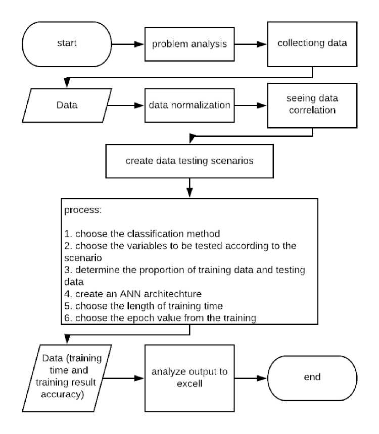
Figure 1. Research Flow Chart
The problem raised is about the selection of features from the most distant or uncorrelated variables to the dependent variable to determine the effect of accuracy and computation time.
The data to be tested is secondary data taken from the UCI Machine Learning Repository which consists of 8124 data units with a total of 22 attributes and one class of classification results. The following are the features of the data.
-
• Edibility
-
• Cap shape
-
• Cap surface
-
• Cap color
-
• Bruises?
-
• Odor
-
• Gill Attachment
-
• Gill Spacing
-
• Gill Size
-
• Gill Color
-
• Stalk Shape
-
• Stalk Root
-
• Stalk Surface above Ring
-
• Stalk Surface below Ring
-
• Stalk Color above Ring
-
• Stalk Color below Ring
-
• Veil Type
-
• Veil Color
-
• Ring Number
-
• Ring Type
-
• Spore Print Color
-
• Population
-
• Habitat
Data normalization is done so that data can be processed in SPSS. The initial data is still in the form of letters representing the data for each feature. Normalization is done by replacing a letter with a certain value.
Correlation testing between data is carried out with the SPSS tool, the first step is to enter the data to be tested for correlation to determine the significance value, this value has a range of 0-1, the features to be removed are those that have a significance value above 0.05 because the value is above the threshold. This limit of significance has a large correlation and does not have a significant impact on the classification results. However, if there is no feature that has a value above 0.05, then the feature with the largest value will be removed.
The test scenario carried out refers to the feature selection to be carried out, which sees the correlation of the features or is also known as the independent variable on the classification result which is the dependent variable because it is bound and affected by the independent variable. The test scenario is done by testing all data first without involving feature selection, and the next step is to start selecting one by one the features with weak or distant correlation.
This study uses the Artificial Neural Network Multilayer Perceptron method. The variables are tested one by one according to the scenario created. ANN architecture with a minimum number of units in hidden layer of 50 and a maximum of 51, the maximum training time is 15 minutes, the maximum epoch given is 1000, and the proportion of training data and test data to be used is 70:30.
The output of this system is a pair of data accuracy and computation time, each of which is 10 because the test is carried out 10 times, the average of the accuracy and the computation time are calculated.
Output analysis was performed in Microsoft Excel. The accuracy and computation time of each scenario are calculated and a graph is then made to represent the calculation results.
The results and discussions that have been carried out will be elaborated one by one starting from data normalization, data correlation test results, making test scenarios in accordance with the results of the correlation test, and finally discussion of the classification results.
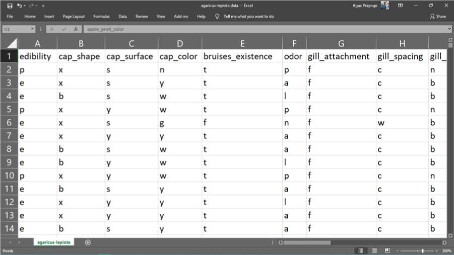
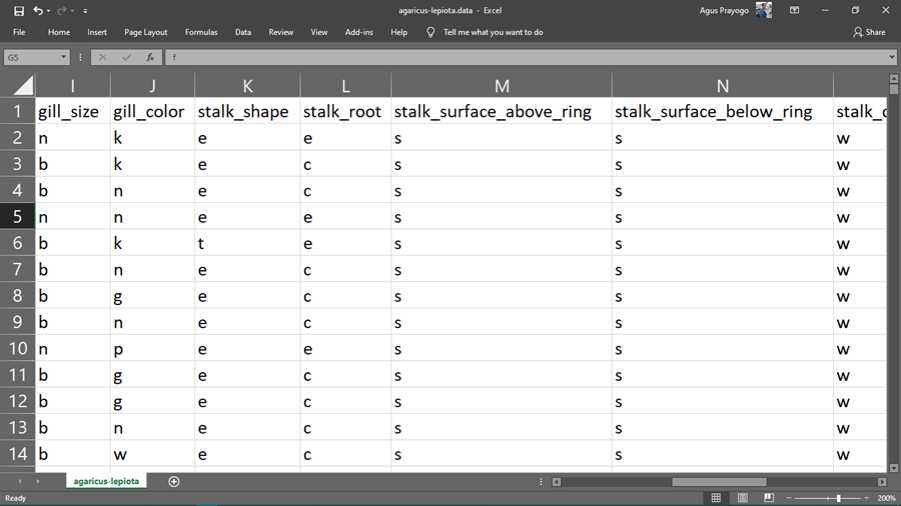
The following is the original data from the Mushroom dataset obtained from the UCI Machine Learning Repository.
|
B ' |
b- c» = |
agaricus-lepiota.data - Excel |
Agus Prayogo ffl |
- |
a × | ||||||
|
File |
Home Insert |
Page |
Layout Formulas I |
Uata Review View Add-ins Help Q |
Tell me what you want to do |
,Q. Share | |||||
|
* | |||||||||||
|
o |
P |
Q |
I |
R |
S |
I T |
■ |
i | |||
|
1 |
stalkcolor |
a |
covering |
Stalkcolorbelowring |
veil_type |
veil |
color |
ringnumber |
ringtype |
spore_pr | |
|
2 |
W |
W |
P |
W |
O |
P |
k | ||||
|
3 |
W |
W |
P |
W |
O |
P |
n | ||||
|
4 |
W |
W |
P |
W |
O |
P |
n | ||||
|
5 |
W |
W |
P |
W |
O |
P |
k | ||||
|
6 |
W |
W |
P |
W |
O |
e |
n | ||||
|
7 |
W |
W |
P |
W |
O |
P |
k | ||||
|
8 |
W |
W |
P |
W |
O |
P |
k | ||||
|
9 |
W |
W |
P |
W |
O |
P |
n | ||||
|
10 |
W |
W |
P |
W |
O |
P |
k | ||||
|
11 |
W |
W |
P |
W |
O |
P |
k | ||||
|
12 |
W |
W |
P |
W |
O |
P |
n | ||||
|
13 |
W |
W |
P |
W |
O |
P |
k | ||||
|
14 |
W |
W |
P |
W |
O |
P |
n | ||||
|
H Sgaritus-Iepiota |
I ® |
I |
■ □ | ||||||||
|
Ready |
M H-- |
—1-1 |
----+ 200% | ||||||||
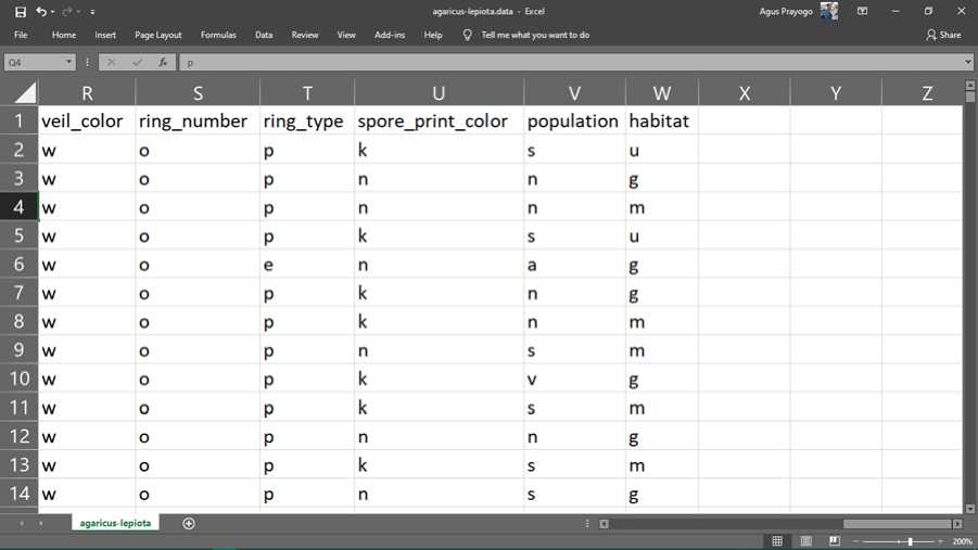
Figure 2. chunks of original data
The data above is a representation of the physical and characteristics of the 8124 mushrooms. Each mushroom has 22 attributes, namely edibility, shape, color, surface, gills, stalk, ring, veil, population and habitat. To simplify data storage, data is stored in abbreviated letters. the following is a description of each of these abbreviations.
|
a. |
Edibility |
: edible = e, poisonous = p |
|
b. |
cap-shape |
: bell = b, conical = c, convex = x, flat = f, knobbed = k, sunken = s |
|
c. |
cap-surface |
: fibrous = f, grooves = g, scaly = y, smooth = s |
|
d. |
cap-color |
: brown = n, buff = b, cinnamon = c, gray = g, green = r, pink = p, purple = u, red = e, white = w, yellow = y |
|
e. |
bruises? |
: bruises = t, no = f |
|
f. |
odor |
: almond = a, anise = l, creosote = c, fishy = y, foul = f, musty = m, none = n, pungent = p, spicy = s |
|
g. |
gill-attachment |
: attached = a, descending = d, free = f, notched = n |
|
h. |
gill-spacing |
: close = c, crowded = w, distant = d |
|
i. |
gill-size : |
broad = b, narrow = n |
|
j. |
gill-color : |
black = k, brown = n, buff = b, chocolate = h, gray = g, green = r, orange = o, pink = p, purple = u, red = e, white = w, yellow = y |
|
k. |
stalk-shape : |
enlarging = e, tapering = t |
|
l. |
stalk-root : |
bulbous = b, club = c, cup = u, equal = e, rhizomorphs = z, rooted = r, missing =? |
|
m. |
stalk-surface-above-ring: |
fibrous = f, scaly = y, silky = k, smooth = s |
|
n. |
stalk-surface-below-ring : |
fibrous = f, scaly = y, silky = k, smooth = s |
|
o. |
stalk-color-above-ring : |
brown = n, buff = b, cinnamon = c, gray = g, orange = o, pink = p, red = e, white = w, yellow = y |
|
p. |
stalk-color-below-ring : |
brown = n, buff = b, cinnamon = c, gray = g, orange = o, pink = p, red = e, white = w, yellow = y |
|
q. |
veil-type : |
partial = p, universal = u |
|
r. |
veil-color : |
brown = n, orange = o, white = w, yellow = y |
|
s. |
ring-number : |
none = n, one = o, two = t |
|
t. |
ring-type : |
cobwebby = c, evanescent = e, flaring = f, large = l, none = n, pendant = p, sheathing = s, zone = z |
|
u. |
spore-print-color : |
black = k, brown = n, buff = b, chocolate = h, green = r, orange = o purple = u, white = w, yellow = y |
|
v. |
population : |
abundant = a, clustered = c, numerous = n, scattered = s, several = v, solitary=y |
|
w. |
habitat : |
grasses = g, leaves = l, meadows = m, paths = p, urban = u, |
waste = w, woods = d
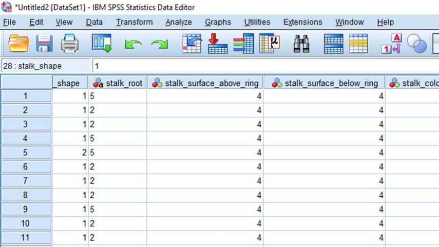
The data is then normalized by changing each data cell from letters to numbers. The following are the results of the data changes.
@ *Untitled2 [DataSet1] - IBM SPSS Statistics Data Editor
File Edit View Data Transform Analyze Graphs Utilities Extensions Window Help
|
: ^^ I^ |
© 85 tΓ- -Si g' |
HS ■ ≡ jj4 ^W L | |||
|
28: stalk_shape 1 | |||||
|
⅛ edibility |
⅛⅛ cap shape |
⅛cap surface |
& cap color |
⅛⅛ bru ses existence | |
|
1 |
0 |
3 |
4 |
1 | |
|
2 |
1 |
3 |
4 |
10 | |
|
3 |
1 |
4 |
9 | ||
|
4 |
0 |
3 |
3 |
9 | |
|
5 |
1 |
3 |
4 |
4 | |
|
6 |
1 |
3 |
3 |
W | |
|
7 |
1 |
1 |
4 |
9 | |
|
8 |
1 |
1 |
3 |
9 | |
|
9 |
0 |
3 |
3 |
9 | |
|
10 |
1 |
1 |
4 |
10 | |
|
11 |
1 |
3 |
3 |
10 | |
O ×

Visible: 23 of 23 Variables
|
Aodor |
Λgi∣∣ attachment |
Aqill spacing |
A qi∣∣ size |
A qi∣∣ color |
A stalk shape |
|
I 7 |
3 |
1 |
2 |
1 |
1 |
|
I 1 |
3 |
1 |
1 |
1 |
1 |
|
T 2 |
3 |
1 |
1 |
2 |
1 |
|
∣ 7 |
3 |
1 |
2 |
2 |
1 |
|
0 |
3 |
2 |
1 |
1 |
2 |
|
I 1 |
3 |
1 |
1 |
2 |
1 |
|
I 1 |
3 |
1 |
1 |
5 |
1 |
|
I 2 |
3 |
1 |
1 |
2 |
1 |
|
I 7 |
3 |
1 |
2 |
8 |
1 |
|
I 1 |
3 |
1 |
1 |
5 |
1 |
|
2 |
3 |
1 |
1 |
5 |
1 |
Visible: 23 of 23 Variables
|
∣r above riπq |
⅛> stalk color below rinq |
⅛⅛ veil type |
veil color |
⅛ riπq number | |
|
8 |
8 |
1 |
3 |
1 | |
|
8 |
8 |
1 |
3 |
1 | |
|
8 |
8 |
1 |
3 |
1 | |
|
8 |
8 |
1 |
3 |
1 | |
|
8 |
8 |
1 |
3 |
1 | |
|
8 |
8 |
1 |
3 |
1 | |
|
8 |
8 |
1 |
3 |
1 | |
|
8 |
8 |
1 |
3 |
1 | |
|
8 |
8 |
1 |
3 |
1 | |
|
8 |
8 |
1 |
3 |
1 | |
|
8 |
1 |
3 |
1 |
O ×

Visible: 23 of 23 Variables
|
⅛⅛ ring number |
A ring type |
⅛ spore print color |
^> populaton |
⅛⅛ habitat | |
|
3 1 |
5. |
4 |
5 |
A. | |
|
3 1 |
5 |
2 |
3 |
1 | |
|
3 1 |
5 |
2 |
3 |
3 | |
|
3 1 |
5 |
1 |
4 |
5 | |
|
3 1 |
2 |
2 |
1 |
1 | |
|
3 1 |
5 |
1 |
3 |
1 | |
|
3 1 |
5 |
1 |
3 |
3 | |
|
3 1 |
5 |
2 |
4 |
3 | |
|
i 1 |
5 |
1 |
5 |
1 | |
|
3 1 |
5 |
1 |
4 |
3 | |
|
3I 1 |
S |
2 |
3 |
1 |
Figure 3. Chunks of normalized data
The following are provisions for changes to each value of the features carried out in the normalization
|
process. | ||
|
a. |
Edibility |
: edible = 1, poisonous = 0 |
|
b. |
cap-shape |
: bell = 1, conical = 2, convex = 3, flat = 4, knobbed = 5, sunken = 6 |
|
c. |
cap-surface |
: fibrous = 1, grooves = 2, scaly = 3, smooth = 4 |
|
d. |
cap-color |
: brown = 1, buff = 2, cinnamon = 3, gray = 4, green = 5, pink = 6, purple = 7, red = 8, white = 9, yellow = 10 |
|
e. |
bruises? |
: bruises = 1, no = 0 |
|
f. |
odor none = 0, pungent = |
: almond = 1, anise = 2, creosote = 3, fishy = 4, foul = 5, musty = 6, 7, spicy = 8 |
|
g. |
gill-attachment |
: attached = 1, descending = 2, free = 3, notched = 4 |
|
h. |
gill-spacing |
: close = 1, crowded = 2, distant = 3 |
|
i. |
gill-size |
: broad = 1, narrow = 2 |
|
j. |
gill-color |
: black = 1, brown = 2, buff = 3, chocolate = 4, gray = 5, green = 6, |
|
orange = 7, pink = 8, purple = 9, red = 10, white = 11, yellow = 12 | ||
|
k. |
stalk-shape |
enlarging = 1, tapering = 2 |
|
l. |
stalk-surface-above-ring |
fibrous = 1, scaly = 2, silky = 3, smooth = 4 |
|
m. |
stalk-surface-below-ring |
fibrous = 1, scaly = 2, silky = 3, smooth = 4 |
|
n. |
stalk-color-above-ring |
brown = 1, buff = 2, cinnamon = 3, gray = 4, orange = 5, pink = 6, red = 7, white = 8, yellow = 9 |
|
o. |
stalk-color-below-ring |
brown = 1, buff = 2, cinnamon = 3, gray = 4, orange = 5, pink = 6, red = 7, white = 8, yellow = 9 |
|
p. |
veil-type |
partial = 1, universal = 2 |
|
q. |
veil-color |
brown = 1, orange = 2, white = 3, yellow = 4 |
|
r. |
ring-number |
none = 0, one = 1, two = 2 |
|
s. |
ring-type |
cobwebby = 1, evanescent = 2, flaring = 3, large = 4, none = 0, pendant = 5, sheathing = 6, zone = 7 |
|
t. |
spore-print-color |
black = 1, brown = 2, buff = 3, chocolate = 4, green = 5, orange = 6, purple = 7, white = 8, yellow = 9 |
|
u. |
population |
abundant = 1, clustered = 2, numerous = 3, scattered = 4, several = 5, solitary = 6 |
|
v. |
habitat |
grasses = 1, leaves = 2, meadows = 3, paths = 4, urban = 5, waste = 6, woods = 7 |
Note that the stalk root feature has missing data, then this feature is removed
Correlation testing was carried out using IBM SPSS Statistic 25 on the classification results, namely the variable result of treatment shown in the table below
¾⅛ *0utput1 [DocumentIJ - IBM SPSS Statistics Viewer
File Edit View Data Transform Insert Format Analyze Graphs Utilities Extensions Window

|
□ |
Correlations bn edibility cap_shape cap_surface cap_color |
|
edibility |
PearsonCorreIation 1 -.199” -.1 87 - 058” Sig. (2-tailed) .000 .000 .000 N 8124 8124 8124 8124 |
|
cap-shape |
PearsonCorreIation -.199" 1 -.007 -.177 Sig. (2-tailed) .000___________________________.525_________.000 N 8124 8124 8124 8124 |
|
cap_surface |
PearsonCorreIation -.187” -.007 1 -.023^ Sig. (2-tailed) ,000__,525_________________________.039 N 8124 8124 8124 8124 |
|
ran rnlnr |
Paarcnn Pnrrolatinn _ ∩ζθ _ 1 77 _ fm 1 |
|
Help | |||||||||||
|
+ | |||||||||||
|
ises_exist ence |
odor |
gill_attachme nt |
gill_spacing |
gill_size |
gill_color |
Stalk-Shape |
stalk-Surface _above_ring |
sta _b | |||
|
.502” |
-.895” |
-.129” |
.348” |
-.54θ" |
.27θ" |
.102" |
.215” | ||||
|
.000 |
.000 |
.000 |
.000 |
.000 |
.000 |
.000 |
.000 | ||||
|
8124 |
8124 |
8124 |
8124 |
8124 |
8124 |
8124 |
8124 | ||||
|
- 200^^ |
.187” |
.032” |
-.06l" |
.259” |
-.069” |
.248” |
- 071” | ||||
|
.000 |
.000 |
.004 |
000 |
.000 |
.000 |
.000 |
.000 | ||||
|
8124 -.020 |
8124 .240” |
8124 -.162" |
8124 -.096” |
8124 .275” |
8124 -.123” |
8124 .037” |
8124 .015 | ||||
|
.078 |
.000 |
.000 |
.000 |
.000 |
.000 |
.001 |
.165 | ||||
|
8124 |
8124 |
8124 |
8124 |
8124 |
8124 |
8124 |
8124 | ||||
|
m*f" |
∩77"" |
1 Qθ"" |
∩9√ |
_ ncn” |
- ∩7∩ |
. ∩1 7 | |||||
¾⅛ 'Output 1 [Document1] - IBM SPSS Statistics Viewer
File Edit View Data Transform Insert Format Analyze Graphs Utilities Extensions Window

|
Ξ |
.attachme nt |
gill_spacing |
gill_size |
gi∣Lcolor |
stalk-Shape |
stalk-Surface _above_ring |
stalk-Surface -LeIoW-Iing |
stalk_color_a bove_ring |
|
-.129” |
348” |
-.54θ" |
.27θ" |
102” |
.215” |
.139” |
.264” | |
|
.000 |
.000 |
.000 |
.000 |
.000 |
.000 |
.000 |
.000 | |
|
8124 |
8124 |
8124 |
8124 |
8124 |
8124 |
8124 |
8124 | |
|
.032" |
-06l” |
.259" |
-.069” |
248” |
-.07l" |
-.069” |
-.O6θ" | |
|
.004 |
.000 |
.000 |
.000 |
.000 |
.000 |
.000 |
.000 | |
|
8124 |
8124 |
8124 |
8124 |
8124 |
8124 |
8124 |
8124 | |
|
-.162” |
-.096” |
.275” |
-.123" |
.037” |
.015 |
.000 |
.251" | |
|
.000 |
.000 |
.000 |
.000 |
.001 |
.165 |
.993 |
.000 | |
|
8124 |
8124 |
8124 |
8124 |
8124 |
8124 |
8124 |
8124 | |
|
1 O')"" |
m√ |
_ ∩□Y" |
_ non |
_ OΛ∩"" |
_ ∩1 7 |
_ m7" |
_ ∩λZ" |

|
stalk_color_b βlowjing |
VeiIJype |
Veiljolor |
ring_number |
ringjype |
spore_printj olor |
populaton |
habitat | |
|
.245" |
b |
-.145" |
.214" |
.360” |
-.519” |
-.299” |
.022' | |
|
.ooo |
.000 |
.000 |
.000 |
.000 |
.000 |
.044 | ||
|
8124 |
8124 |
8124 |
8124 |
8124 |
8124 |
8124 |
8124 | |
|
-.057" |
b |
.037” |
-.069" |
- 307” |
.251” |
ij29" |
134” | |
|
.000 |
.001 |
.000 |
OOO |
OOO |
.000 |
OOO j | ||
|
8124 |
8124 |
8124 |
8124 |
8124 |
8124 |
8124 |
8124 | |
|
.26θ" |
b |
-.155" |
.060" |
-.208” |
.310” |
-.189” |
-.192” | |
|
.000 |
.000 |
.000 |
.000 |
.000 |
.000 |
.000 | ||
|
8124 |
8124 |
8124 |
8124 |
8124 |
8124 |
8124 |
8124 | |
|
. m«" |
b |
1 QQwr |
∩ι n |
1 'h" |
. ∩0∩" |
. ∩1 Q |
. ∩α∩" |
Figure 4. Correlation Test Result
The meaning of the star symbol ** there indicates that the variable has the strongest closeness or correlation with Edibility, and the sig. (2-tailed) value, 000 which means it has a significant correlation. From the data above, it can be seen that all features have a very strong correlation with edibility. All correlations are worth 000, apart from habitat. Because this feature has the lowest correlation, this feature correlation will be tested.
The test scenario carried out is based on the results of the correlation or the relationship between the independent variables and the dependent variable, namely the results of the edibility classification so that the scenario can be translated into:
-
a. testing involves all variables
-
b. testing involves all variables except habitat
Data is processed in the IBM SPSS Statistic 25 Tool, using an Artificial Neural Network Multilayer Perceptron and produces the following accuracy and computation time.
Table 1. Calculation of The Test Scenario
|
Trial to- |
Involves all variables |
without habitat | ||
|
accuracy |
time |
accuracy |
time | |
|
1 |
100% |
80 |
100% |
91 |
|
2 |
100% |
70 |
100% |
70 |
|
3 |
100% |
1.03 |
99.90% |
57 |
|
4 |
100% |
61 |
100% |
75 |
|
5 |
100% |
59 |
100% |
70 |
|
6 |
100% |
54 |
100% |
70 |
|
7 |
100% |
1.06 |
99.80% |
33 |
|
8 |
100% |
81 |
100% |
59 |
|
9 |
100% |
61 |
100% |
71 |
|
10 |
100% |
38 |
100% |
78 |
average 100% 50.609 99.97% 67.4
The table above is part of the calculation of predetermined scenarios along with the results of the average accuracy and computation time obtained.
The analysis obtained from the results of the average accuracy and time of this classification test is that the accuracy reaches 100% in a scenario using all data. Then, the accuracy decreased to 99.97% in scenarios without habitat features. The computation time in the scenario uses all data as high as 50 milliseconds, then increases 67 milliseconds in the scenario without habitat features. This is of course caused by the loss of habitat features. Although the habitat feature is the only feature that correlates the worst, this feature still has a strong enough correlation in determining the edibility feature. Even so, there are still 21 other features that have a very strong correlation, so that the accuracy does not decrease drastically.
Research on feature selection on the Mushroom dataset to test its effect on accuracy and computation time has been successfully carried out. With the proportion of the number of training data and test data 70:30 in the form of percent, using the help of IBM SPSS Statistic 25 data, the data gets the accuracy by performing a feature selection scenario that is worse than accuracy without selecting features, getting 99.97% accuracy while a scenario without feature selection gets 100% accuracy. In terms of both accuracy and computation time, the changes did not change significantly.
References
-
[1] Schlimmer, Jeff. (27 April 1987). Mushroom Data Set Retreived from https://archive.ics.uci.edu/ml/datasets/Mushroom
-
[2] Kusuma, Angga. 2015. Jamur / Fungi. Lampung: Lampung University.
-
[3] Cambridge Dictionary. (2020). Classification. Retrieved October 10, 2020 from
https://dictionary.cambridge.org/dictionary/english/classification
-
[4] Ottom, Mohammad Ashram. (October 2019). Classification of Mushroom Fungi Using Machine Learning Techniques. Retrieved November 4, 2020 from
https://www.researchgate.net/publication/337024220_Classification_of_Mushroom_Fungi_Using_ Machine_Learning_Techniques/link/5e259c2592851c067e221f78/download
-
[5] Gorianto, Frisca Olivia. (November 2019). Breast Cancer Classification Using Artificial Neural Network and Feature Selection. Retrieved November 5, 2020 from
https://ojs.unud.ac.id/index.php/JLK/article/view/51874/32618
128
Discussion and feedback