Diagnosis of Heart Disease Using Generalized Learning Vector Quantization (GLVQ) and Genetic Algorithms Methods

Jurnal Ilmu Komputer VOL. XIII No. 1

p-ISSN: 1979-5661

e-ISSN: 2622-321X

Diagnosis of Heart Disease Using Generalized Learning Vector Quantization (GLVQ) and Genetic Algorithms Methods

Made Dwi Ariyawan¹, I Gede Arta Wibawa², Luh Arida Ayu Rahning Putri³

• ^1,2,3 Program Studi Teknik Informatika, Fakultas Matematika dan Ilmu Pengetahuan Alam, Universitas Udayana

Jl. Kampus Bukit Jimbaran (80361), Badung, Bali, Indonesia

¹dwi.aryawan55@gmail.com

²gede.arta@unud.ac.id

³luh.arida@cs.unud.ac.id

Abstract

Coronary heart disease is one of the diseases that contributes quite high rates of death in the world. The World Heart Federation estimates that the number of deaths due to coronary heart disease in Southeast Asia reached 1.8 million cases in 2014. In 2013 there were at least 883,447 people diagnosed with coronary heart disease in Indonesia with the majority of patients aged 5564 years. The death rate due to heart disease is quite high, which is about 45 percent of all deaths in Indonesia. Therefore this study was conducted in the hope of reducing the number of deaths caused by heart disease and the concrete steps that could be made to the diagnosis results by the system.

In this study using a combination of two methods, namely Genetic Algorithms and Generalized Learning Vector Quantization (GLVQ). The combination of these methods is done to get the optimal weight in the training process which later the weight is used to get the classification results in the testing process

From the test results obtained an average accuracy 71.50% with the best parameters namely learning rate 0.02, reduction learning rate (dec α) 0.9, epoch 100, population number 30, number of generations 20, crossover rate 0.2, and mutation rate 0.1.

Keywords: Genetic Algorithms, Generalized Learning Vector Quantization, Heart Disease

were only two class labels taken which were worth 1 if the patient was healthy and worth 2 if the patient was sick.

	Table 1. Heart Disease Data
No	Age Sex Cpt Rbp Chol Fbs Re Mhr Exa Op Slp Ca    Thal     T
1 2 3	70   1.0   4.0   130   322    0    2.0    109    0    2.4   2.0    3.0     3.0       2 67    0    3.0   115   564    0    2.0    160    0    1.6   2.0     0      7.0       1 57   1.0   2.0   124   261    0     0     141    0    0.3   1.0     0      7.0       2
268 269 270	56    0    2.0   140   294    0    2.0    153    0    1.3   2.0     0      3.0       1 57   1.0   4.0   140   192    0     0     148    0    0.4   2.0     0      6.0       1 67   1.0   4.0   160   286    0    2.0    108   1.0   1.5   2.0    3.0    3.0       2

• 2.2.    Data Processing Process

For the initial training process (training), it starts with randomization of initial weights which is -0.5 to 0.5. After randomization of initial weights, do crossovers and mutations to produce offspring or child (solution). After producing an individual (child), evaluate the fitness value of the individual (child) through the Generalized Learning Vector Quantization (GLVQ) method. Individuals (children) with the best fitness will be maintained. The process stops when it reaches the specified number of generations. After reaching the specified number of generations it will produce the best weights which will later be used by the testing process to get the classification results. After getting the classification results, then calculate the accuracy value.

Figure 1. Research Flowchart

• 2.3.    Training Process

The training process must be done first in order to find the final weights that will later be used in the testing process (testing). Data training flowchart can be seen in the figure 2. Explanation of Figure 2 as follows:

• 1.    The input matrix consists of 189 training data, input population numbers, number of generations, crossover rate (Cr), mutation rate (Mr), learning rate, reduction in learning rate, and epoch.

• 2.    Defining the maximum epoch, learning rate, number of generations, and initial weight. The initial weight used in this study is random numbers -0.5 to 0.5.

• 3.    Awaken the initial population, parent selection, then do the process of crossing (crossover) and mutation to get a new individual. In this study, the crossing process is carried out using the singlepoint crossover method and at the mutation stage is carried out by selecting 2 genes from each child to exchange values. After that enter the GLVQ method.

• 4.    The training process with the GLVQ algorithm will continue to repeat and stop when the maximum epoch. The result of GLVQ training is accuracy which is used as a fitness value.

• 5.    Fitness value determines whether or not an individual passes from the selection process. In this study, the fitness value used is the accuracy of the GLVQ training process [7].

• 6.    The process of selection, reproduction, and evaluation will continue to repeat until reaching the maximum generation which will later produce the best weight where the weight will be used in the testing process.

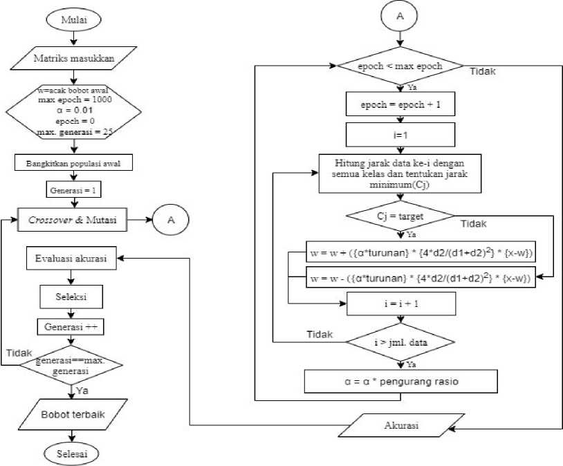
Figure 2. Training Flowchart

• 2.4.    Testing Process

Testing is a process of classifying heart disease using weights that have been obtained in the previous training process. Flowchart data testing can be seen in figure 3.

The testing process begins by entering the testing data, amounting to 81 data and the best weight that has been obtained in the training process. Then it will be processed using the GLVQ method. This method will calculate the distance of the input data to each class and later will find the smallest distance as a result of the classification of heart disease.

• 2.5.    System Interface Design

In the process of designing a system interface, the tools used are tools Tkinter which is a GUI library (graphical user interface) owned by Python. Tkinter itself is a library that is directly bundled in Python and works according to the toolkit owned by Python. In this study, the purpose of making a system interface design is to facilitate the user in operating the application for diagnosing heart disease. In designing the interface, there are 3 main components including the training process (training), the testing process (testing), and the process of diagnosing heart disease. In the training process (training) there are 3 input buttons to enter the value of the parameters used and 1 button to start training (training). The results obtained in the training process (training) is the accuracy of training and weights that will be used in the testing process (testing) which is stored in excel form, the appearance of the training process can be seen in Figure 4. In the testing process (testing), the weight load that has been obtained from the training process (training), start the testing process by clicking the "Check accuracy" button. After the testing process (testing) is complete, the system will display the accuracy obtained from the process, the appearance of the testing process can be seen in Figure 5. Then there is the process of diagnosing heart disease, in this process there are 13 features that will be manually inputted by the user. After inputting 13 features, click the "Diagnosis" button to get the classification results, the diagnosis process can be seen in Figure 6.

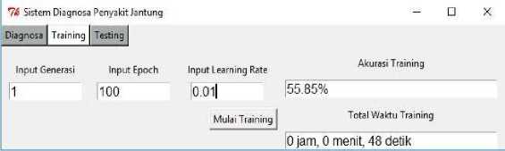
Figure 4. Display Training Process on The System

• 7^ SistemDiagnosaPenyakitJantung                       —     □

Diagnosa ∣ Training ∣ Testing ∣

Akurasi Testing

I             .∣   55.0%

Load Bobot CekAkurasi I

Total Waktu Testing

O jam, 0 menit, 2 detik

Figure 5. Display Testing Process on The System

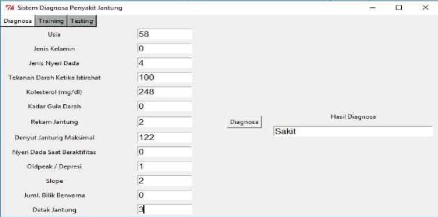
Figure 6. Display Diagnostic Process on The System

• 3.    Result and Discussion

  • 3.1.    Learning Rate Testing Results and Analysis

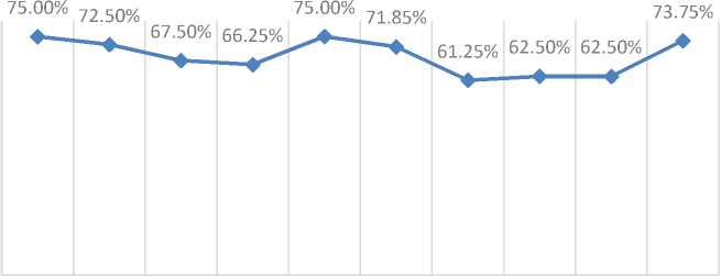
Tests carried out with variations in learning rates 0.01, 0.02, 0.03, 0.04, 0.05, 0.06, 0.07, 0.08, 0.09, 0.1 by using the number of epoch as much as 100 times, reducing the learning rate (dec α) 0.9, the total population of 100, the number of generations 1, crossover rate 0.2, mutation rate 0.1 to find the most optimal learning rate.

LEARNING RATE

Figure 7. Learning Rate Testing Results and Analysis

Figure 7 shows the lowest accuracy obtained at the learning rate value of 0.03, the learning rate value of 0.05, 0.06 produces a stable accuracy of 67.50% and 0.08, 0.09, 0.1 produces a stable accuracy of 66.25%. The most optimal learning rate is 0.02 with the highest accuracy of 73.75%.

• 3.2.    Learning Rate Reduction Testing Results and Analysis

Reduction of learning rate affects the value of learning rate (α) in the process of updating weights so that it will also affect the results of accuracy. At this stage, testing is done with a reduction in learning rate (dec α) 0.1, 0.2, 0.3, 0.4, 0.5, 0.6, 0.7, 0.8, 0.9 using the learning rate parameter 0.02, the number of learning (epoch) 100 times, the number of populations 100, the number of generation 1, crossover rate 0.2, and mutation rate 0.1 to find the most optimal dec α value. The results and analysis of reducing learning rate testing (decα) can be seen in figure 8.

LEARNING RATE REDUCTION TESTING RESULTS AND

76.00%

74.00%

72.00%

70.00%

68.00%

66.00%

64.00%

62.00%

60.00%

58.00%

56.00%

0.01   0.02   0.03   0.04   0.05   0.06   0.07   0.08   0.09

LEARNING RATE REDUCTION

Figure 8. Learning Rate Reduction Testing Results and Analysis

Figure 8 shows the lowest accuracy which is 60% obtained from the reduction value of learning rate (dec α) 0.1 and the highest accuracy obtained from the reduction value of learning rate (dec α) 0.9 by 75%. After getting the optimal value of the learning rate and the reduction in learning rate (dec α), the next step is to find the optimal value of the epoch.

• 3.3.    Epoch Testing Results and Analysis

At this stage, testing is done with variations of epoch 100, 200, 300, 400, 500, 600, 700, 800, 900, 1000 using the learning rate parameter (α) 0.02, reducing the learning rate (dec α) 0.9, the total population of 100 , number of generation 1, crossover rate 0.2, and mutation rate 0.1 to find the optimal epoch. The results and analysis of reducing learning rate testing (decα) can be seen in Figure 9.

EPOCH TESTING RESULTS AND ANALYSIS

80.00%

70.00%

60.00%

δ 50.00% <

⊃ 40.00%

30.00%

20.00%

10.00%

0.00%

100   200   300   400   500   600   700   800   900   1000

EPOCH

Figure 9. Epoch Testing Results and Analysis

Figure 9 shows the lowest accuracy of 61.25% obtained from the amount of learning (epoch) as much as 700 times, accuracy experienced stable at epoch 800 and 900 and the highest accuracy of 75% at epoch 100 and 500. Because epoch 100 and 500 have accuracy values that are same, then in the next stage, the epoch used is epoch 100 to save time.

• 3.4.    Results and Analysis of Testing Population Amounts

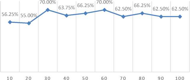
Tests carried out with variations in values of populations 10, 20, 30, 40, 50, 60, 70, 80, 90, 100, the parameters used are learning rate 0.2, reduction learning rate 0.9, learning (epoch) 100 times, number of generations 1 , crossover rate 0.2, and mutation rate 0.1 to find the most optimal population. The results and analysis of population testing can be seen in figure 10.

RESULTS AND ANALYSIS OF TESTING POPULATION AMOUNTS

80.00%

70.00%

60.00%

U 50.00%

<

⊃ 40.00%

^ 30.00%

20.00%

10.00%

0.00%

POPULATION AMOUNT

Figure 10 shows the accuracy has increased and decreased with increasing population. The lowest accuracy of 55% is obtained from a population of 20 and the highest accuracy of 70% is obtained from a population of 30 and 60. In the next stage the total population used is 30.

• 3.5.    Results and Analysis of Testing Generation Amounts

Tests carried out with variations in values of 5, 10, 15, 20, and 25 using other parameters include learning rate 0.02, reduction learning rate 0.9, epoch 100, population number 30, crossover rate 0.2, and mutation rate 0.1 to find the number of generations the most optimal. The results and analysis of testing the number of generations can be seen in figure 11.

RESULTS AND ANALYSIS OF TESTING GENERATION

80.00%

70.00%

60.00%

U 50.00% <

§ 40.00%

30.00%

20.00%

10.00%

0.00%

5

15           20           25

GENERATION AMOUNT

Figure 11. Results and Analysis of Testing Generation Amounts

Figure 11 shows the change in accuracy at each increase in the number of generations is not very significant. The lowest accuracy of 60% is obtained from the number of generations 10 and the highest accuracy of 73.75% is obtained from the number of generations 20. After getting the most optimal number of generations, the next step is to find the optimal value of the crossover rate.

• 3.6.    Results and Analysis of Crossover Rate Testing

The test was carried out with variations in the value of the crossover rate of 0.1, 0.2, 0.3, 0.4, and 0.5 using other parameters namely learning rate 0.02, reduction of learning rate 0.9, epoch 100, total population 30, number of generations 20, mutation rate 0.1. The results and analysis of crossover rate testing can be seen in figure 12.

Figure 12. Results and Analysis of Crossover Rate Testing

In the results and analysis of the crossover rate test shown in figure 12, the increase and decrease in accuracy. The lowest accuracy of 63.75% is obtained from the crossover rate of 0.1 and 0.5 and the highest accuracy of 73.75% is obtained from the crossover rate of 0.2. After getting the most optimal crossover rate, the next step is to find the optimal value of the mutation rate.

• 3.7.    Results and Analysis of Mutation Rate Testing

The test was carried out with variations in the value mutation rate of 0.1, 0.2, 0.3, 0.4 and 0.5 using other parameters is learning rate 0.02, reducing learning rate 0.9, epoch 100, population number 30, number of generations 20, crossover rate 0.2. The results and analysis of mutation rate testing can be seen in figure 13.

RESULTS AND ANALYSIS OF MUTATION RATE TESTING

76.00%

74.00%

72.00%

δ 70.00%

68.00%

o 66.00%

64.00%

62.00%

60.00%

0.1           0.2           0.3           0.4           0.5

MU7ATION RATE

Figure 13. Results and Analysis of Crossover Rate Testing

Figure 13 shows the accuracy has decreased and increased where it has decreased at mutation rates 0.2 and 0.3 and has increased at mutation rates 0.4 and 0.5. The lowest accuracy is 65% at a mutation rate 0.3 and the highest accuracy is 73.75% at a mutation rate 0.1.

• 3.8.    Testing the Best Parameters

After getting the best parameters including learning rate 0.2, reduction of learning rate 0.9, epoch 100, population number 30, number of generations 20, crossover rate 0.2, and mutation rate 0.1 will be re-tested 5 times to try to get an average accuracy. The best parameter test results can be seen in figure 14.

RESULT AND ANALYSIS OF BEST PARAMETERS

• 73.00%      72.50%                                                   72.50%

• 72.50%       ⅜.>

• 72.00%∕

^71.25%       71.25%

• > 71∙50%                    _{t            t}

S 71.00%

3 70.50%                                                 70.00^r

• < 70.00%^<

69.50%

69.00%

68.50%

FIRST      SECOND      THIRD      FOURTH      FIFTH

EXPERIMENT EXPERIMENT EXPERIMENT EXPERIMENT EXPERIMENT

Figure 14. Result and Analysis of Best Parameters

Figure 14 shows the lowest accuracy obtained in the fourth experiment with 70% accuracy and the highest accuracy obtained in the first and fifth experiments. The average accuracy obtained from all experiments using the best parameters is 71.50%.

• 4.    Conclusion

The conclusion obtained from this study is that the more training processes are carried out, the greater the chance of getting the best weight because each process of training the weight obtained is always different. In the testing process, the average accuracy obtained is 71.50% with the best parameters namely learning rate 0.02, reduction learning rate (dec α) 0.9, epoch 100, population number 30, number of generations 20, crossover rate 0.2, and mutation rate 0.1. Based on research references conducted by [1] where the research diagnoses heart disease using a combination of Genetic Algorithm and Backpropagation methods can be compared with research by the author because of the same case but the method used is different namely the merging of Genetic Algorithms and Generalized Learning Vector Quantization (GLVQ). In a study conducted by (Andriana, 2017) an average accuracy of 96% was obtained which is far better than the research conducted by the writer who obtained an average accuracy of 71.50%.

References

• [1]    Andriana A., 2017, Peningkatan Akurasi Jaringan Saraf Menggunakan Algoritma Genetika, Independent Investor Publishing.

• [2]    Arniantya R., Setiawan B.D., dan Adikara P.P., Optimasi Vektor Bobot Pada Learning Vector Quantization Menggunakan Algoritme Genetika Untuk Identifikasi Jenis Attention Deficit Hyperactivity Disorder Pada Anak, Jurnal Pengembangan Teknologi Informasi dan Ilmu Komputer, Vol. 2, No.2, hlm. 679-687, 2018.

• [3]    Hasan Z.F., Hussein A.A., Heart Disease Classification By Genetic Algorithm, Journal of Babylon University, Pure and Applied Sciences, No.9, Vol. 24, 2016.

• [4]    Hermawan I., Pengembangan Sistem Pengenalan Wajah Menggunakan Metode Generalized Learning Vector Quantization, STMIK AMIKOM Yogyakarta, ISSN: 2302-3805, Vol 3.7, No. 61, 2015.

• [5]    Prasetyo E. B., Penerapan Algoritma Genetika dan Jaringan Saraf Tiruan Pada Penjadwalan Mata Kulia di Fakultas Matematika dan Ilmu Pengetahuan Alam Universitas Gadjah Mada, Yogyakarta: Universitas Gadjah, 2014.

• [6]    Ratnasari, et al., Komordibitas Pada Anak Gangguan Pemusatan Perhatian Dan Hiperaktivitas (GPPH) Pada 20 Sekolah Dasar Di Manado, Manado: s.n., 2016.

• [7]    Rismala R., Sulistyo M.D., Penerapan Teknik Klasifikasi Pada Sistem Rekomendasi Menggunakan Algoritma Genetika, Jurnal Ilmiah Teknologi Informasi Terapan, Volume II, No 3, Bandung, 2016.

• [8]    Saputra R.A., Pasrun Y.P., and Basyarah A.N., Macular Edema Classification Using SelfOrganizing Map and Generalized Learning Vector Quantization, Jurnal Ilmu Komputer dan Informasi, 7/2, hlm. 54-60, Surabaya, 2014.

• [9]    Saputro H. A., Mahmudy W. F. dan Dewi C., Implementasi Algoritma Genetika Untuk Optimasi Penggunaan Lahan Pertanian, DORO: Repository Jurnal Mahasiswa PTIIK Universitas Brawijaya vol. 5, no. 12, 2015.

• [10]    Septiari N. W. D., Muliantara A., Widiartha I. M., Pengenalan Aksara Bali Menggunakan Metode Modified Direction Feature dan Algoritma Generalized Learning Vector Quantization, Jurnal Ilmu Komputer Universitas Udayana, Bali, 2015.

64