Threshold Panel Method for Analysis of the Effect of Banking Investment Allocation on Banking Performance, A Cross Country Studies: Some OECD Countries

pISSN : 2301 – 8968

JEKT ♦ 15 [1] : 179-196

eISSN : 2303 – 0186

Threshold Panel Method for Analysis of the Effect of Banking Investment Allocation on Banking Performance, A Cross Country Studies: Some OECD Countries

Mahjus Ekananda

Abstract

The direction of globalization and the integration of the financial system continues to increase in line with the trend of increasing capital flows which is the focus of discussion in this research. This study applies panel data analysis to analyze banking behavior to improve its performance. The analysis uses a linear model and a threshold model—panel data from 1991 to 2020 in 39 countries. Threshold panel regression is a non-linear model applied in this study to prove a change in the impact of independent variables that affect banking performance in specific regimes. In general, the linear model Coef.icients are as expected according to the theory. Analysis using threshold panel regression will give more profound results and higher intuition. Threshold panel regression has a smaller SSR value than the linear model. This study applies one threshold value to produce two different regimes. Changes in the impact occur at a certain threshold. Conclusively, this study finds threshold values for GDP growth, Concentration, Inflation, Leverage, Efficiency, and Credit Allocation. The GDP growth rate as a threshold is the most efficient model. The Coef.icients on the threshold panel regression model generally are in line with theoretical expectations. Still, some differences become the advantages of this non-linear model, revealing different economic conditions.

Key words : bank performance, panel threshold regression, capital, credit allocation

JEL : G20, C24, E22, E51

Background

Lane & Milesi-Ferretti (2010) studied the cross-border economy and the severity of the 2008-2009 global recession. The results explain that the severity of the global recession is related to pre-crisis macroeconomic and financial factors. They found that pre-crisis levels of development, increasing private credit-to-GDP ratios, current account deficits, and openness to trade helped understand the intensity of the crisis.

In a fast economic condition, the demand for credit will increase, while in a recession, the demand for credit will decrease significantly. Credit demand follows the theory of the pro-

cyclical relationship between economic growth and credit (Afanasyeva and Güntner, 2015). In boom conditions, banks tend to relax lending standards and provide loans to customers with high and low credit risk. Meanwhile, banks will be more careful in a recession and even rationing in lending.

The problem regarding credit allocation has been carried out by Cai (2021). He obtained substantial evidence that expansionary monetary policy will lead to the misallocation of bank credit to less productive firms. Other analyzes show that credit misallocation is partial. More productive companies will take different actions than companies that are not productive. More productive companies had

hoarded cash before the crisis, while less productive companies had invested more in financial assets.

Several researchers convey various conclusions regarding the factors that affect credit allocation and banking profits, showing that these factors' influence on banking performance is not always the same. The level of the variable scale determines change. Aisen & Franken (2010) show that the higher the level of leverage indicates, the more vulnerable the banking system is to the impact of the crisis.

Demirguc-Kunt, et al. (2004) explains that the more concentrated the banking system indicates, the more substantial the market position and the more significant the impact on banking profits. Several structural factors that will affect credit allocation and banking performance include investment share and sectoral structure in an economy—the greater the investment opportunities of a country, the more significant the impact of banking performance. Likewise, more excellent investment opportunities will increase the impact of banks' lending to the corporate sector. However, on the other hand, high growth in the service sector in developed countries will reduce investment demand in developing countries (Summers, 2013).

Some literature mentions several external factors, including trade openness and foreign capital flows. The greater trade openness will increase the impact of a country's investment. Likewise, foreign capital inflows will also encourage investment and demand for corporate credit in the tradable sector through export receipts (Lucas, 1990), (Blanchard & Giavazzi, 2002). Based on observations, an increase in capital flows can also increase property loans in a country (Samarina & Bezemer, 2016).

Several researchers, including Samarina & Bezemer (2016), explain how trade openness

and foreign capital flows increase a country's investment. (Blanchard & Giavazzi, 2002) put more emphasis on inflow behavior. Foreign capital inflows will also encourage investment and demand for corporate credit in the tradable sector through export receipts. Based on the explanation of the background, it can be seen that the relationship between economic variables has a different relationship to the allocation of bank credit, including capital inflows. (IMF, 2017) states that the impact of capital inflows, especially in the form of portfolio investment and debt investment, on credit growth is still ambiguous. On the one hand, the development of capital inflows can be an incentive to increase investment (saving constrained economy). However, at the same time, it can increase the allocation of consumer credit, increasing the vulnerability of financial system stability (investment constrained economy). Previous empirical studies are limited and have not provided a consistent answer on how capital inflows affect banking performance.

The process affects banks' shift in credit allocation, primarily when associated with the increasingly integrated global financial system. In general, the research that has been conducted tends to analyze the allocation of bank credit in terms of banking behavior (micro/internal factors), while other factors of a macro nature, such as trade openness and capital inflows, are still limited. In addition, research on the impact of capital inflows is generally related to the credit boom and is limited to using total capital inflow data. Meanwhile, different compositions and types of capital inflows will impact economic growth, investment, and bank credit (IMF, 2017).

The inter-country economy is part of global capital flows, which cannot be separated from capital flow activities in direct investment and portfolio investment. One factor that influences the allocation of domestic credit disbursement by banks is the inflow of foreign

capital into the banking and corporate sectors (Samarina & Bezemer, 2016). Capital inflows (non-FDI) will increase credit growth for individual and corporate loans. Igan (2015) has conducted this research using data from 1980-to 2011 in various OECD countries.

After the global financial crisis (Global Financial Crisis) 2007-2008, the performance and allocation of bank credit continues to show improvement, especially in personal loans. The trend of shifting in the allocation of bank credit, which is marked by high growth in the individual sector, has generated considerable attention. The phenomenon of high growth in the private sector can increase macroeconomic vulnerability and negatively impact the economy. The negative impact is the inhibition of economic growth, disruption of economic stability, and the emergence of a country's financial system fragility (financial fragility). (Beck, Büyükkarabacak, Rioja, & Valev, 2012); and (Dunn & Ekici, 2006) studied that the decline in credit for the corporate sector accompanied by an increase in personal credit would impact the decline in savings rates and a slowdown in economic growth.

Some studies that have been conducted so far generally analyze the performance of banks from the inner side, such as banking capacity, interest rates, and credit risk. Analysis from the external side, such as trade openness and capital inflows, is still relatively limited (Bezemer, Samarina, & Zhang, 2017). However, not many studies examine the allocation of credit to the banking sector.

Based on the description above, the analysis in this study is focused on testing the hypothesis that capital inflows in the corporate sector affect the decline in bank lending in the corporate sector. In other words, the flow of the model in the corporate sector will shift the source of its capital which was originally obtained from bank credit to capital originating from abroad. The final result is a

decrease in banking profits derived from credit.

Based on the description above, to complete the existing gap and to contribute to the previous literature, this research is focused on looking at the allocation of bank credit associated with the characteristics of the country based on the level of globalization of its financial system (share of foreign banks to total national banking). This is based on the fact that several kinds of literature still show ambiguous results on the impact of foreign banks on domestic credit growth and bank profitability (Claessens & Horen, 2014).

This study was conducted to empirically answer and contribute to the previous literature by providing an integrated approach to examining the relationship between capital inflows and global banking credit allocation using the panel data equation model from 1990-to 2016. This research hypothesizes a relationship between the variables of capital inflows to the level of banking profits.

Theoretical background

We assume the sources come from three economic sectors: banks, firms, and households. The relationship between these three sectors can be explained from the supply and demand side. On the demand side, the condition of corporate and individual balance sheets and the availability of external funds are factors that influence the demand for credit for the corporate and individual sectors. Meanwhile, on the supply side, capital inflows (external funding), macroeconomic conditions, and banking sector characteristics are factors that influence the supply of credit to the corporate and individual sectors. Each sector can be described as follows. The private sector (h) will allocate its income for consumption (Cons1, Cons2) and for saving S

in the form of deposits in the bank Dh and securities (bonds) Bh, and will maximize its utility function by considering budget constraints:

Max U(Cons1, Cons2)

Constraints : Cons1 + Bh + Dh = ω1, pCons2 = Пf + Пb + (1+r) Bh + (1+rD) Dh,

where ω1 represents the initial endowment of consumption, p is the price of Cons2, Пf and Пb are a company and bank profits, r and rD are interest rates earned on bonds and deposits. The corporate sector (f) has the option to invest at the level I, and the source of financing can be obtained from Lf bank credit and by issuing securities Bf, and the corporation will maximize profit:

Max Пf

Constraints : Пf = pf(I) – (1+r)Bf – (1+rL)Lf,

I = Bf + Lf,

Where f is the production function and rL is the bank loan interest rate. The banking sector (b) will choose the supply of credit Lb, demand for deposits Db, and the issuance of bonds Bb, to maximize performance (profit):

Max Пb

Constraints : Пb = rL Lb - rBb – rDDb, Lb = Bb + Db,

In order to optimize credit allocation, banks will take into account the difference between the interest rate for consumer/personal loans and the interest rate for corporate loans (se = r – r*). It is assumed that these two types of credit have substitute properties. Bank credit supply is a function of bank deposit and interest rate differential, l = g(d, se). l is the supply of credit, d is the deposit, and se is the difference in interest rates for consumption

and corporations (Sophocles, Garganas, & Hall, 2012).

The main factors that are considered for credit requests by the corporate and individual sectors include the cost of credit, namely credit interest rates and economic activity. On the supply side, the ability and willingness to lend by banks is influenced by the condition of the sources of funds owned by banks (bank equity, total assets, deposits, and cost of external financing), banking capital position, costs of other alternative bank portfolios (eg, the difference between interest rates). Lending rates and T-bill rates), competition with other banks, and perceived risk (macroeconomic variables, non-performing loans) (Sophocles, Garganas, & Hall, 2012).

Empirical Overview

Domestic Flow of Capital and Credit

Much literature examines the relationship between capital inflows and bank credit. Aoki, Benigno, & Kiyotaki (2009) report a strong relationship between asset prices and credit. In another case, Calderon & Kubota (2012) explain the relationship between capital inflows and credit growth. Capital flows tend to lead to a credit boom. Capital inflows will encourage an increase in asset prices and loosen credit constraints. Mendoza & Terrones (2012) explain this in their research. Industrialized countries and emerging market economies (EMEs) have increased gross capital inflows over 15 years. They found that domestic factors played a much more significant role. Several factors include that overvalued currencies in terms of credit growth tend to attract massive capital inflows. Strong growth and abundance of natural resources are vital in attracting foreign capital

inflows into emerging market economies. In the end, capital inflows will affect credit allocation. Changes in credit allocation will affect bank performance.

Igan & Tan (1995) researched the effect of capital inflows, credit growth, banking performance, and the financial system. They use data from 33 countries from 1980 to 2011. Their research results show that capital inflows will increase credit growth in developing countries. Novelty research by Igan & Tan (1995) divided the composition of capital inflows into two. Capital inflows came from FDI and other inflows. Net other inflows were proven to encourage credit growth and credit booms in the individual and corporate sectors. On the other hand, Net FDI inflows had no significant effect on credit growth.

In general, the behavior of banks in lending is determined by various factors, both internal and external factors of the bank. These factors include bank capacity, interest rates, bank perceptions of risk, and macroeconomic conditions. These factors do not always stand alone but also interact to influence bank behavior in improving banking performance.

Internal factors (bank characteristics)

(Aisen & Franken, 2010) explains that the return on equity or return on equity or profitability of own capital contained in the bank shows that the efficiency of the use of own capital or the better level of profitability of the bank will encourage greater access for banks to increase lending, but also indicates that the bank will face a higher risk.

Han, Zhang, and Greene (2018) studied the relationship between bank market concentration and banking affecting three small firm liquidity sources (cash, lines of

credit, and trade credit). Their research found that in highly concentrated banking markets, small firms hold less cash, have less access to credit lines, are more likely to be financially constrained, and use larger amounts of more expensive trade credit. We also find support for banking relationships. Banking relationships increase tiny business liquidity, particularly in highly concentrated banking markets. They were reducing the adverse effect of market concentration of banks stemming from market forces.

Several researchers have investigated the relationship between Loan Portfolio Concentration and Bank Stability. Kusi et al. (2019) specifically investigated the linearity and non-linearity effects of sectoral loan concentration on bank stability.The sectoral concentration of bank lending has a non-linear shape effect on bank stability in Ghana. They argue that although sectoral loan concentration can weaken bank stability in the short term, lending concentration can increase bank stability in the long term. From their findings, policymakers, regulators, and bank managers should design policies or regulations that prohibit sectoral lending concentration. Policymakers should also include plans and policies that encourage banks to develop core competencies and competitive banking advantages. Weller (2009) conducted a study using the Federal Reserve Survey data. Weller's (2009) study looks at financial constraints, the cost of credit, and some contributions to the cost of credit, including the sources and types of loans. Weller's (2009) study suggests that discrimination based on taste and structural discrimination may have persisted and may have increased over time. The gap in access to credit costs will affect optimal banking profits. Banks must maintain

optimal access to credit to affect better banking performance.

Research Methods

The data that will be used in this research is panel data, a combination of cross-section and time-series data. Greene (2018) explains

several advantages of using panel data: paying attention to heterogeneity, more complete information, less possibility of collinearity between the variables studied, and data having more degrees of freedom and efficiency. The data used are from 39 countries for 30 years (1991-2020).

Table 1. Variable List

Variable	Description	Unit	Remarks
CrAllit	Measure the share of non-financial business loans to total bank loans	%     total kredit	BIS (Bank            for International Settlements)
BInit	Measure the share of inflows entering the banking to total GDP	% GDP	BoP – IMF
NBInit	Measure the share of inflows entering the non-bank to total GDP	% GDP	BoP – IMF
Conit	Measure the concentration. concentration is calculated from the total share of the top 5 largest bank assets to total banking assets	% total aset	World Bank
Effit	Measure the efficiency that is calculated from the ratio of total revenue to costs	%	World Bank
GDPperCapit	Label for GDP per capita	USD	World Bank
InflSit	Inflation is calculated from annual CPI growth	% (yoy)	IMF - WEO
Erateit	The exchange rate of local currency units) against the U.S. dollars	LCU/USD	IMF - IFS
Levit	Measure the ratio of total bank credit to total deposit	%	World Bank
Deregulit	The deregulation index is the average of all components, with an index of 1 – 10.	Index	Fraser Institute’s Economic Freedom Indicators
ROEit	Return on Equity	%   before tax	Bank Dunia

The model used refers to the framework of thought and empirical studies that have been carried out by Samarina & Bezemer (2016). Our research analyzes the impact of credit allocation and other factors on banking performance. In this study, the data used are annual in several countries (globally) for 30

years (1990-2020). The selection of the period is based on the heterogeneity of the data. The countries included in this study include 39 countries.

We discussed banking performance during an increasingly integrated global financial system

situation. In this regard, this study will analyze the close relationship between capital inflows and bank credit allocation. In addition to capital flows, we also include bank characteristics (Bezemer & Zhang, 2017). The dynamics of bank performance are also considered so that the inter-period banking profit linkage becomes strong. Data analysis was conducted using secondary data obtained from several sources, including IMF, BIS, CEIC, BPS, Bank Indonesia, and World Bank data.

The use of explanatory variables refers to the theoretical framework as described in the theoretical background. The capital inflows variable consists of capital originating from the banking sector (BIni_t) and the corporate

sector (NBIni_t). Some researchers use the division of capital inflows, including Some researchers use the division of capital inflows, including Lane & Milesi-Ferretti (2010), Afanasyeva and Güntner (2015), Cai (2021), Barnes, Lawson, and Radziwill (2010), Calderón & Kubota (2019) and Igan & Tan (1995).

Bank internal variables that describe banking behavior, namely banking concentration (Soydan, & Kara (2020), Sufian & Habibullah (2010), Han et al. (2015), and Kusi et.al (2019). Sdiscussion about banking leverage (Mendoza, Jorge Eduardo & Calderon, Cuauhtemoc (2006), and efficiency banking Spyros, Eleni, & Helen (2014)). In general, the equations used are as follows (Model I):

ROE_it = a + β₁CrAll_it + β₂dBIn_i,_t + β₃dNBIn_i,_t + β₄Con_it + β₅dLev_it + β₆GDPperCap_it + β₇dInfls_it + β₈dLnErate_it + β₉Deregul_i,_t + e_it

(1)

ROE variable is bank return on equity (% before tax). Banking concentration (Con), is the share of the 5 largest banks' assets to total domestic banking assets. Leverage (Lev), is the ratio of lending to bank deposits. Efficiency (Eff), is the ratio of banking costs to income, and the control variables consist of income level (real GDP per capita, based on constant prices in 2005 USD), inflation rate (yoy, %), money market deregulation index, and exchange rate ( against USD). The NFC variable is the share of corporate sector credit to the total credit disbursed by banks. The capital inflow variable consists of the capital inflow variable to the banking sector (BIn) and the non-bank sector (NBIn).

Some of the advantages of using panel data are that panel data can accommodate unobserved individual heterogeneity; panel

data can reduce collinearity between variables; and estimating panel data can minimize bias, Ekananda (2019) and Wooldridge. (2002). The first advantage of a model with a threshold is that there are different regimes for the same data and model. The second advance of this model, threshold regression, can show the significance of the causality relationship under different threshold regimes, which cannot be demonstrated if we use interactions between variables. The third advantage of the dynamic Threshold Panel estimation method is that it uses panel data where dynamic processes and heterogeneity of economic variables occur. The following equation gives the standard regression estimation model with panel data thresholds with individual-specific effects (Wang, 2015) for a single threshold model.

yn - μ + ^χitti⅛ < ^γ)^β₁ + ^χitti⅛ ≥ ^γ)^β₂ +u_i + ε_it,

(2)

For multiple threshold models

yit- μ + Xittiit < Y1)β₁ + Xittiι≤Qit < Y2)β₂ + ^xittiit ≥ Y2)β₃ + Ui + ε_u,

(3)

Where the independent variable can be shifted according to the regime which is determined by as the threshold value.

^yit^-μ+ ^xittiit^{, γ})^β +Ui + ^εit^,

(4)

Where Xit(Qit.Y) ^- (^ >^) and β ^- Cβ1β2)'

(5)

Given , estimator : β — {X*(γ)'X*(γ)]~¹ X*(γ)'y*

The estimator determines the value that minimizes the Residual of Sum Square (RSS). The process of selecting the method applies to Hansen (1999), where it is a consistent estimator for, then we can form a statistical likelihood-ratio (LR) test as follows:

LRi(Y)

LRι(γ) - LRi(Y) σ²

(6)

Measurement of significance level for LR significance test. The value of the quantile is calculated from the following inverse function:

c(α) — —2 log(1 — √1- α)

(7)

If LR₁(γ) exceeds c(α), we can reject H0. Where the hypothesis for the single-threshold model is

H0 : β1 = β2 dan H1 : β1 ≠ β2

According to our research, the panel threshold regression can be developed by applying a dynamic model using the GMM estimator on the threshold model. This study uses the estimator proposed by Seoa, Kim & Kim (2019). Under the restriction of the dynamic model, the research equation (Model II, equation 1) becomes:

ROE_it — α_i + (β₁CrAll_it + β₂dBIn_i,_t + β₃dNBIn_i,_t + β₄C0n_it + β₅dLev_it +

β₆GDPperCap_it + β₇dInfls_it + β_βdLnErate_it + β₉Deregul_it)Kk_it≤ ~γ) + (διCrAll_it + δ₂dBIn_i,_t + δ₃dNBIn_i,_t + δ₄Con_it + δ₅dLev_it + δ₆GDPperCap_it + δ₇dInfls_it + δ₈dLnErate_it + δ₉Deregul_it)Kk_it> ~γ) + ε_it

(8)

Result and discussion                       Cointegration Test to the Data Series: ROE,

CrAll, BIn, NBIn, Con, Lev, Eff and

Table 2 shows the results of the panel data GDPperCap. Null Hypothesis:    No

cointegration test. The table shows the long- cointegration, indicating the Newey-West term balance and correction of the automatic bandwidth selection and Bartlett cointegrated variables. Kao Residual kernel.

Table 2 t-Statistic Prob.

ADF        -7.406366  0.0000

Residual variance   257.7989

HAC variance    91.90057

Nonlinearity testing is applied in the study. Smooth Threshold Remaining Nonlinearity Tests are applied in the research process to ensure that the threshold setting on the model

b1*s [ + b2*s^2 + b3*s^3 + b4*s^4 ]. We use Terasvirta Sequential Tests. Tests are based on the third-order. The Null Hypothesis H03: b1=b2=b3=0.

is correct. Taylor expansion alternatives : b0 +

Table 3. Linearity Tests

Threshold	F	d.f.	p-value	Linear model
Infls	5.956582 *)	(8, 1136)	0.0000	Rejected +)
Con	5.438441 *)	(8, 1150)	0.0000	Rejected +)
Lev	6.572206 *)	(9, 1149)	0.0000	Rejected +)
GDPperCap	6.572206 *)	(9, 1149)	0.0000	Rejected +)
Eff	9.178511 *)	(8, 1150)	0.0000	Rejected +)
*) original model is	rejected at the 5% level using H03. +) at the 5% level using H03.

Table 3 explains that the application of the threshold can be made. The test results of all threshold variables indicate that the linear model is rejected. If we use a linear equation, the Coef.icients show a nonlinear impact. Nonlinear impact (threshold regression) can be interpreted that the impact of the independent variable is not the same for all data conditions. The threshold application can

be made to explore the impact of changes in the condition of the threshold variable.

The proper method will produce more efficient estimated econometric equations. The size of the sum square of residual (SSR) is used to determine a more efficient method (Ekananda, 2018). Table 4 and Table 6 summarize the SSR values of the various methods used in the study.

Table 4. The comparison between linear methods

	Commod Effect	Fixed Effect	Random Effect
SSR	286,125.5	236,292.2	257,935.6
R2	0.056993	0.333785	0.073702

Summary for Hausman test

	Chi-Sq. Statistic	Chi-Sq. d.f.	Prob.
Cross-section random	35.607112	9	0.0000

Note : based on equation (A)

Table 4 shows SSR and R2 in a linear model, namely common effect (CE), fixed effect (FE), and random effect (RE). The more restrictive the model has, the greater the SSR value in the linear model. The individual effect model is lower than the common effect

model. The results of the Hausman test show that the best model is the fixed effect. The model selection results to strengthen the research process will focus on threshold regression that applies fixed effects.

Table 5. Estimation Results for the linear model

Variable	Expec. Sign	CE		FE		RE
		Coef.	t-Stat	Coef.	t-Stat	Coef.	t-Stat
C		15.098	5.808	20.770	5.438	17.701	2.393
CrAll	-	-0.052	-2.005	-0.404	-8.654	-0.259	-5.151
dBInfl	+	0.083	3.542	0.084	3.331	0.120	3.172
dNBInfl	-	0.000	0.077	-0.001	-0.340	-0.002	-0.554
Con	+	-0.066	-4.045	-0.079	-3.166	-0.107	-3.196
dLev	+	0.060	2.213	0.063	2.560	0.152	1.975
dGDPCap	+	0.000	3.960	0.000	2.435	0.001	3.286
dInfls	+	0.001	0.860	0.001	1.032	0.001	0.561
dLnExRate	-	-2.437	-1.881	-4.347	-3.211	-1.328	-0.494
Deregul	+	0.456	1.592	1.550	3.506	1.426	1.603
SSR		286,125.5		236,292.2		257,935.6
R2		0.056993		0.333785		0.073702
Fstat		7.789		11.960		10.255

The estimation results for the linear model are shown in Table 5. In general, the variables that correspond to the expected sign are credit allocation (CrAll), Capital Inflow to the bank (BIn), Concentration, Leverage (Lev), GDPperCap, and an exchange rate (Erate), and deregulation. All variables show a significant effect on the common effect, fixed effect, and random effect models. The variables NBIn and Infls (Inflation) did not show a significant effect. We can conclude that changes in the variables do not result in a definite change in ROE. The result of model selection shows that the best model I is a fixed effect.

The estimation results show that the SSR for fixed effects is the smallest. There are more significant variables than the common effect and random effect equations. The impact of

exchange rate depreciation (Erate) reduces ROE. The research developed Model II by applying several threshold variables as. The linearity test value shows that all Model II indicates non-linearity (Table 3). We can notice that the SSR of the linear model (Table 4) is more significant than that of the nonlinear model (Table 6). SSR in the Linear model is quite varied. This study will discuss several models with various thresholds. We choose several variables for analysis; the study selects several thresholds, namely GDP per Cap, efficiency, concentration, credit allocation, leverage, and inflation. The smallest SSR is the model with a GDPPerCap threshold, and the largest SSR is Inflation. Some software chooses the best model is the smallest SSR value, but this study will analyze all thresholds to be explained analytically.

Table 6. The comparison of SSR and threshold value

Variable	Threshold	CI *)	SSR	F1 stat
GDPPerCapita	2,096.188	[2,096.19, 2,100.35]	213,480.4	161.069
Efficiency (Eff)	79.97	[49.35, 80.84]	221,109.8	116.486
Concentr (Con)	72.895	[71.14, 73.36]	221,279.5	115.529
Cred Alloc (CrAll)	22.0762	[22.08, 22.08]	223,500.8	103.14

Leverage (Lev)	67.611	[64.08, 70.3]	227,979.9	118.108
Inflation (Infls)	-0.121	[-0.12, 0.01]	229,881.3	68.886

*) CI : Confidence Interval (95%)

Table 6 explains that model II with GDPPerCap threshold has the smallest SSR compared to other variables. Threshold values describe the high and low regime limits. The linearity test checks whether the parameter can apply to all data or whether there is a change in the parameter at a specific threshold value. The linearity test significantly rejected the valid parameters for all data. This test reflects that the stability of the parameters can not be maintained. The linear model (Model I) is seen as a restriction of the non-linear model (Model II). Table 7 summarizes the threshold measurement results compared to the average value and the 50% percentile value.

The following are descriptive statistics of the panel variables used and consist of the average value, standard deviation, and Coef.icient of variation value as reflected in Table 4.1, which displays a statistical summary sample with a total of 1,053 observations, with 39 countries and 39 periods from the years 1990 – 2020. Globally, the average allocation of corporate bank credit is 40.83% (total credit), with the share of capital inflows in the non-

bank sector being more extensive than the share of capital inflows in the banking sector.

The Std Dev value indicates a variable with a level of volatility or a tendency to change. The larger the value, the more the variable is the most volatile. Based on Table 7, changes in capital inflows in the banking (bin) and nonbank sectors (nbin) are the most volatile. This capital indicates that the volatility of capital inflows is higher, which indicates that capital inflows tend to be short term.

The Table 7 escribes descriptive statistics of the main research variables divided into several periods, especially considering the financial crisis in 1997-1998 and 2007-2008, namely the period 1990-1998, the period 1999-2007, and the period 2008-2016. Meanwhile, capital inflows in the banking sector showed an increasing trend until the 1999-2007 period but declined again in the 2008-2020 period, with a lower share of capital inflows than capital inflows in the nonbank sector. On the other hand, capital inflows in the non-bank sector have the highest share, with an increasing trend.

Table 7. The comparation between threshold value, average and pecentile 50%.

Variable	Standard Dev	Average	Percentile (50%)	SSR	Threshold Value
Infls	31.57	11.43	2.52	212,407.24	8.52
Conc	14.53	75.01	76.22	198,387.48	72.89
NBIn	966.19	204.92	29.88
Lev	40.25	100.46	94.95	212,679.34	64.01
CrAlloc	10.55	39.86	37.44	223,500.8	29.03
GDPperCap	18,541.18	26,047.67	28,068.99	196,770.89	4574.02
BIn	218.55	85.50	27.57
Eff	8.71	58.23	59.76	216,298.91	49.35
ROE	5.76	11.06	11.37
Erate	1,393.32	323.51	2.09
Deregul	0.99	8.41	8.58

Almost all selected threshold values (Inflation, Concentration, Leverage, Credit Allocation, GDPperCap, and Efficiency) are equal to average and percentile at 50%. Estimation of the threshold value is based on changes in the

impact of two groups of high and low variables. Estimation with threshold regression has better intuition because it analyzes the regression according to the high and low of certain variables.

Tabel 8. Estimation Results for non-linear models, GDPperCap and Concentration as threshold

		GDPperCap				Concentration
Variable	sign	Lower		Up	per	Lower		Up	per
		Coef.	t-Stat	Coef.	t-Stat	Coef.	t-Stat	Coef.	t-Stat
CrAll	-	1.241	1.340***	-0.384	-9.459***	-0.475	-5.999***	-0.405	-6.684 ***
dBInfl	+	0.877	0.196	0.119	3.264***	0.045	3.879***	0.218	3.331***
dNBInfl	-	0.868	0.573	-0.003	-0.884	0.002	1.236**	-0.012	-1.984 ***
Con	+	-0.138	-0.647	-0.056	-1.847 **	-0.159	-2.532 ***	-0.188	-2.699 ***
dLev	+	2.784	1.668**	0.069	2.539***	0.227	2.290***	0.101	2.056***
dGDPCap	+	0.262	0.556	-0.343	-6.149 ***	0.001	2.808***	0.001	2.393***
dInfls	+	0.057	1.368**	0.001	5.233***	0.001	0.295	1.768	1.386***
dLnExRate	-	0.652	0.978	0.000	0.060	-4.144	-2.305 ***	-5.872	-0.659
Deregul	+	0.019	1.350*	-0.003	-1.391*	0.948	1.015*	1.136	1.315*
Gamma		4574.02				72.89
SSR		213,480.400				221,279.510
Fstat		161.069				115.529

Table 8 of the estimation results of GDPperCap (left) and Concentration (right) as threshold variables. CAlloc, BIn, NBIn, Leverage, Efficiency, GDPperCap, and Deregul affect ROE significantly and are in line with the expected sign. Estimation with threshold regression produces the impact of each variable differently.

In countries with high GDPperCap, more significant independent variables than those with low GDPperCap. The effect of independent variables on ROE can be estimated according to the theoretical model. In countries with high GDPperCap, the Coef.icient value of the independent variable is higher than in those with low GDPperCap. We can conclude that countries with high GDPperCap are more responsive to the impact of independent variables than those with low GDPperCap. In general, the effect of independent variables on ROE can be estimated according to the theoretical model.

The independent variable has significantly more impact than banking at a low concentration level in banking with a high concentration level. From both models, changes in the exchange rate do not show a significant impact. This exchange rate is because the depreciation variable in various countries does not effectively affect banking performance. Conclusively increasing efficiency will increase.

The study applies inflation as a reference threshold value (Table 9). High inflation will cause economic contraction and slowdown. High inflation causes prices to rise and causes the economy to contract. In banking in countries with high inflation, almost all Coef. icients show significance and follow the expected sign. There are many Coef.icients in banking in low-inflation countries which show insignificant. Changes that occur in the share of inflows entering the non-bank sector to total GDP (dNBInfl), Concentration, (Concr) Leverage (Leve), and GDP growth

(dGDPCap) will not lead to an increase in performance. The empirical results prove that changes in banking performance are more responsive in conditions of higher inflation.

The decrease in the independent variable causes the opposite direction. The high inflation situation must be kept under control under the policy direction.

Tabel 9. Estimation Results for non-linear models, Inflation and Leverage as threshold

Inflation                                 Leverage

Variable	sign	Lower		Upper		Lower		Upper
		Coef.	t-Stat	Coef.	t-Stat	Coef.	t-Stat	Coef.	t-Stat

CrAll	-	-0.647	-2.579***	-0.418	-9.311 ***	-0.108	-0.513	-0.399	-8.325 ***
dBInfl	+	0.603	4.928***	0.101	4.305***	0.051	3.318***	0.267	3.712***
dNBInfl	-	-0.272	-4.342 ***	-0.001	-0.320	0.001	0.470	-0.102	-1.957 ***
Con	+	-0.130	-1.008	-0.134	-2.587 ***	-0.079	-0.945	-0.138	-3.612 ***
dLev	+	0.218	0.836	0.144	2.059***	0.739	1.367*	0.075	2.225***
dGDPCap	+	0.000	-0.051	0.000	4.444***	0.001	3.393***	0.001	3.863***
dInfls	+	1.415	1.119*	0.002	0.935	-0.046	-1.267 *	0.000	0.169
dLnExRate	-	-5.487	-0.195	-2.898	-1.200 *	10.222	0.886	-4.422	-1.582 **
Dereg	+	1.781	1.328*	1.051	1.619**	0.511	0.661	1.595	2.253 ***
Gamma		8.52				64.01
SSR		229,881.279				227,979.930
Fstat		68.886				118.108

In Table 9 on the right, the threshold value is Leverage. Leverage is calculated as the bank's total credit ratio to the total deposit. The higher the Leverage, the greater the total credit compared to deposits. There is no difference in the estimation results between the leverage levels. According to the theory, all variables CAlloc, BIn, NBIn, Leverage, Efficiency, GDPperCap, and deregulation affect ROE.

Table 10 shows the Efficiency variable as the threshold. Efficiency is calculated from the ratio of total revenue to costs. High efficiency reflects banking income which is higher than banking operational costs. Banking management and strategy have increased the bank's revenue beyond its costs. At high efficiency, efficiency is greater than the effect of efficiency at low efficiency. Several main variables also show an impact on ROE following the theory.

Tabel 10. Estimation Results for non-linear models

		Efficiency				Credit Allocation
Variable	sign	Lower		Upper		Lower		Upper
		Coef.	t-Stat	Coef.	t-Stat	Coef.	t-Stat	Coef.	t-Stat
CrAll	-	-0.355	-8.739 ***	-0.214	-1.099	-1.081	-0.513	-0.401	-6.723
dBInfl	+	0.125	3.312***	0.248	1.856**	-0.168	-0.289	0.126	3.367
dNBInfl	-	-0.004	-1.075	-0.010	-1.093 *	1.690	1.135	-0.003	-1.003
Con	+	-0.102	-1.998 ***	-0.305	-2.269 ***	0.171	0.766	-0.122	-3.086
dLev	+	0.118	1.706**	0.474	2.368***	2.293	1.303	0.089	2.779
dGDPCap	+	0.001	4.685***	0.000	0.044	-0.000	-0.107	0.001	4.140
dInfls	+	0.002	0.956	0.436	1.362*	0.029	1.493	0.001	0.462
dLnExRate	-	-1.774	-0.765	-10.027	-0.537	2.377	0.285	-4.486	-2.264
Deregul	+	1.684	2.118***	0.792	0.393	1.061	0.250	2.127	2.543
Gamma		49.35				29.03
SSR		221,109.786				223500.783
Fstat		116.486				103.14

The variable share of non-financial business credit to total bank credit (CrAll) is applied as a threshold because at high CrAll, nonfinancial business credit is increasingly dominant as an element of bank credit (Table 10 right). Loans disbursed for non-financial businesses are getting bigger. In the portion where CrAll is high, the impact of the independent variable is generally significant. Banking performance will immediately respond to changes that occur in the independent variables. On the other hand, at low CrAll, changes in the independent variables are not immediately responded to by banking performance.

The policy implications of the research are explained as follows. The measurement of the threshold value adds to the analysis of the regression results. Generally, a threshold value proves that there is a change in the economic environment under the threshold variable being reviewed (Hansen, 1999). In several studies, threshold regression can optimize policy because it is adjusted to the prevailing regime. The measurement results show that one country can pass through 2 different regimes, which should have 2 different policies (Afanasyeva, Elena and Güntner, Jochen, 2015).

Table 11. Frequency of data at specific Threshold values

(1)      (2)	(3)      (4)	(5)      (6)	(7)       (8)	(9)     (10)	(11)    (12)
CrAll 29.03	Con 72.89	Lev 64.01	Eff 49.35	GDPCap 4574.02	Inf 8.52
Cntry.   Freq. ARGE   19 GREE   30 INDO   20	Cntry.   Freq. ARGE  24 BRAZ   21 CHIL   13 COL-   17 INDI    22 INDO   29 ITAL   21 JAPA   30 LUX-   24 MEX-   15 POLA   21 RUSS   29 THAI   16 TURK   15 US    30	Cntry.   Freq. ARGE   14 BELG   12 HKON  18 INDI    11 JAPA   19 LUX-   30 TURK   16 UK    30	Cntry.   Freq. HKON  23 INDI    23 IREL    23 LUX-   20 NORW  12 SING   23 THAI    18 TURK   14	Cntry.   Freq. COL-   16 INDI    30 INDO   30 RUSS   14 SAFR   13 THAI   19 TURK   12	Cntry.   Freq. ARGE   20 HUNG   11 INDI    12 INDO   11 RUSS   20 TURK   24

Through non-linear regression results, we can obtain a threshold value that divides the data into 2 parts of the high and low-value regime—the total number of 39 countries and time from 1991 to 2020 (30 periods). Table 11 shows countries with data frequencies below the threshold (low-value regimes). All data below the threshold (column 1 to column 10), except for the last column (column 11 and column 12) is a list of countries with inflation

values higher than the threshold number (high inflation regimes). The countries listed in Table 11 are mostly developing countries. Developed countries located in high-value regimes are outside this table.

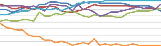
If we compile the data of the high-value regime, we find something interesting to analyze. Figure 1 shows the frequency of data arranged according to time. Most of the data

are in the high-value regime. More countries showing that high inflation data decreases— are in high-value regimes than low-value more and more countries with low inflation.

regimes. Exceptions occur in inflation data,

Figure 1. Frequency of Data in the High-Value Regime.

40.00

35.00

30.00

25.00

20.00

15.00

10.00

5.00

0.00

o^ζ5 <£ ,& .Φ <P Φ <$> ,Φ _aΦ _nΦ ^    & Λ^ς^ ^^θ

^^^^^^CrAll ^^^^^^ Leve ^^^^^^ Concr ^^^^^^^ Effic ^^^^^nGDPCap «■■■■■■B Inf

The Concentration graph shows an increasing trend, especially from 2013 to 2020—many countries with high concentrations. GDPCap data shows increasing frequency. In a high GDPCap regime, more and more countries have a high GDPCap. Even though the population grows, GDP can compensate until the GDPCap value also increases. The increase in productivity in the last 10 years has shown its effect on the development of capital and credit flows through the banking sector. These results follow the research of Afanasyeva, Elena, and Güntner (2015). Economic developments in the construction and consumption sectors triggered the increase in bank credit. After the economic revival and capital flows after the 2008 financial crisis, inflation is back to being competitive and countries experiencing financial crises are recovering. Bezemer, D., Samarina, A., & Zhang, L. (2017) reported the results of their research that the more open capital flows, the direct flow of funds to the real sector were able to shift the role of bank credit.

Support for low economic costs is getting higher. The inflation chart shows a downward trend. Countries with high inflation (in high inflation regimes) are fewer. Low inflation in most countries increases capital gains in the financial sector, thereby increasing banks' competitiveness and operational efficiency in various countries. Sufian and Habibullah (2010) report the results of their research that Bank-specific, Industry-specific, and Macroeconomic Determinants influence banking efficiency.

Conclusions

This study produces exciting conclusions about how the internal banking and macroeconomic variables affect performance at various levels of specific regimes. The direction of globalization and the integration of the financial system continues to increase in line with the trend of increasing capital flows which is the focus of discussion in this research. By using the panel data equation, the

results of the analysis can be concluded as follows:

According to the theory, the Coef.icients of the linear model and the threshold panel regression are as expected. Threshold panel regression produces a smaller SSR compared to the linear model. Threshold panel regression proves a change in the impact of independent variables that affect banking performance in specific regimes.

Conclusively, this study analyzes the threshold values for GDP growth, Concentration, Inflation, Leverage, Efficiency, and Credit Allocation. The GDP growth rate as a threshold is the most efficient model. Analysis of the model with the level of GDP growth, the results obtained where the high GDP growth sensitivity of the independent variable is more than the low GDP growth regime.

The research results on the linear model indicate that, in general, the level of capital inflows in the non-bank sector (NBIn) does not affect the allocation of bank credit. However, the Threshold panel regression results and NBIn measurement impact particular Concentration, Inflation, Concentration, and Efficiency regimes. The results of this study explain that the increase in non-bank capital inflows (NBIn) does not significantly impact banking performance.

The share of non-financial business credit to total bank credit (CrAll) reduces banking performance. An increase in Credit Allocation means that non-financial business credit will reduce banking income. This fact applies to all analyses of linear models and threshold regression models.

On the micro side, the variable bank characteristics that significantly affect banking performance is the level of banking leverage, namely the percentage of lending to bank deposits. Lending to bank deposits indicates that the ability of banks to disburse credit is increasing along with the increase in capital

inflows received, especially in the banking sector.

Some control variables contained in the equation also show significant results, especially for variables of per capita income, deregulation, and exchange rates. The variable of income per capita has a significant effect on the allocation of bank credit with a positive relationship. Meanwhile, the deregulation variable has a significant positive effect on the allocation of bank credit.

References

Afanasyeva, Elena and Güntner, Jochen, 2015, Lending Standards, Credit Booms, and Monetary Policy, No 15115, Economics Working Papers from Hoover Institution, Stanford University.

Aisen, A., & Franken, M. 2010. Bank credit

during the 2008 financial crisis: a crosscountry comparison. International Monetary Fund Working Paper, No.10/47.

Aoki, K., Benigno, G., & Kiyotaki, N. 2009. Capital Flows and Asset Prices. CEP Discussion Papers.

Barnes, Sebastian., & Lawson, Jeremy., and Radziwill, Artur., 2010. "Current Account Imbalances in the Euro Area: A Comparative Perspective," OECD Economics Department Working Papers 826, OECD Publishing. DOI: 10.1787/5km33svj7pxs-en

Beck, T., Büyükkarabacak, B., Rioja, F. K., & Valev, N. 2012. Who Gets the Credit? And Does It Matter? Household vs. Firm Lending Across Countries. The B.E. Journal of Macroeconomics, Volume 12, Issue 1.

Bezemer, D., Samarina, A., & Zhang, L. 2017. The shift in bank credit allocation: new data and new findings. DNB Working Paper, 559.

Blanchard, O., & Giavazzi, F. 2002. Current

account deficits in the Euro area: The end of the Feldstein-Horioka puzzle? Brookings Papers on Economic Activity, 2.

Calderón, César & Kubota, Megumi, 2019. "Ride the Wild Surf: An investigation of the drivers of surges in capital inflows," Journal of International Money and Finance, Elsevier, vol. 92, pages 112-136. DOI: 10.1016/j.jimonfin.2018.11.007

Cai, Yue, 2021. "Expansionary monetary policy and credit allocation: Evidence from China," China Economic Review, Elsevier, vol. 66. DOI: 10.1016/j.chieco.2021.101595

Claessens, S., & Horen, N. V. 2014. Foreign Banks: Trends and Impact. Journal of Money, Credit and Banking Volume 46 Issue s1, 295326.

Demirgüç-Kunt, Asli, Laeven, Luc and Ross Levine, 2004, “Regulations, Market Structure, Institutions, and the Cost of Financial Intermediation.” Journal of Money, Credit and Banking, 36 (3 Pt.2), 593-622.

Ekananda, M., 2018, Miss-Invoicing Analysis In Asean-China Free Trade Aggrement (ACFTA), European Research Studies Journal Volume XXI, Issue 1, p. 187-205

Ekananda, M., 2019, The Analysis of The Effect of Non-Bank Sector Investment to The Bank Credit Allocation, The Asia-Pacific Research in Social Sciences and Humanities Conference 2018 – Universitas Indonesia, BOOK Chapter,   Nova   Science

Publishers, Inc, Section 3, Chapter 14, ISBN: 978-1-53616-276-9

Greene, William H 2018, Econometric Analysis, ISBN:  0134461363,  9780134461366  ,

eighth Edition, Pearson 2018, New York.

Han, Liang., Zhang, Song and Greene, Francis J., 2015, Bank market concentration, relationship banking, and small business liquidity, Article first published online: December 28, 2015; Issue published: June 1, 2017, Volume: 35 issue: 4, page(s): 365384.

https://doi.org/10.1177/0266242615618733

Hansen, B. E. 1999, Threshold Effects in NonDynamic Panels: Estimation, Testing, and Inference, Journal of Econometrics, pp. 345368.

Igan, D., & Tan, Z. 1995. Capital Inflows, Credit Growth, and Financial Systems. IMF Working Paper. 19 Aug 2015, SBN: 9781513581262

IMF. 2017. Increasing Resilience to Large and Volatile Capital Flows: The Role of Macroprudential Policies, Press Release No. 17/260, For Immediate Release, July 5, 2017, International Monetary Fund, 700 19th Street, NW, Washington, D.C. 20431 USA

Kusi, Baah Aye., Adzobu, Lydia., Abasi, Alex Kwame., and Ansah-Adu, Kwadjo., 2019, Sectoral Loan Portfolio Concentration and Bank Stability: Evidence from an Emerging Economy, Volume: 19 issue: 1, page(s): 6699, Article first published online: December 9, 2019; Issue published: April 1, 2020, https://doi.org/10.1177/0972652719878597

Lane, Philip R & Milesi-Ferretti, Gian Maria, 2010, The Cross-Country Incidence of the Global Crisis, IMF Economic Review volume 59,  pages77–110. Published: 23

November 2010

Lucas, J. R. 1990. Why doesn't capital flow from rich to poor countries? The American Economic Review, Vol 80, No.2.

Mendoza, Jorge Eduardo & Calderon, Cuauhtemoc, 2006. "Impactos regionales de las remesas en el crecimiento económico de México [Regional impacts of remittances on the economic growth of Mexico]," MPRA Paper 3331, University Library of Munich, Germany, revised Sep 2006.

Samarina, A., & Bezemer, D. 2016. Do Capital Flows Change Domestic Credit Allocation? Journal of International Money and Finance.

Seoa, Myung Hwan, Kim, S., and Kim, Y., 2019, Estimation of Dynamic Panel Threshold Model using Stata, Department of Economics, Seoul National University, bDepartment of Economics, University of Maryland, Department of Economics, Hongik University, February 28, 2019.

Sophocles, N. B., Garganas, E. N., & Hall, S. G. 2012. Consumer credit in an era of financial

liberalisation: An overreaction to repressed demand? MPRA Paper No.41819.

Soydan, Aylin., & Kara, Serap Bedir., 2020. "Implications of Capital Flows for Domestic Credit Growth: Evidence from Panel Data Analysis," Eurasian Journal of Economics and Finance, Eurasian Publications, vol. 8(4), pages 231-245.

Spyros, P., Eleni, K., & Helen, L. 2014. Bank leverage and return on equity targeting: intrinsic procyclicality of short-term choices. Bank of Greece Working Paper.

Sufian, Fadzlan and Habibullah, Muzafar Shah ,2010, Bank-specific, Industry-specific and Macroeconomic Determinants of Bank Efficiency: Empirical Evidence from the Thai Banking Sector, The Journal of Applied Economic Research, vol. 4, 4: pp. 427-461. , First Published December 17, 2010.

Summers, L. 2013. Speech at the 14th annual IMF research conference: Crises yesterday and today.

Wang, Q. 2015 Fixed-effect panel threshold model using Stata, Institute of Statistics and Econometrics, Nankai University, Tianjin, China, The Stata Journal, 15, Number 1, pp. 121–134.

Weller, Christian E.,  2009, Credit Access, the

Costs of Credit and Credit Market Discrimination,  The Review of  Black

Political Economy, Volume: 36 issue: 1, page(s): 7-28,  January 1, 2009;  Issue

published:      January      1,      2009.

https://doi.org/10.1007/s12114-009-9034-6

Wooldridge. 2002. Econometric Analysis of Cross Section and Panel Data. MIT Press.

196