The Dynamics of Exchange Rate, Inflation, and Trade Balance in Indonesia

ISSN : 2301-8968

Vol. 14 No.2, Agustus 2021

EKONOMI

KUANTITATIF

TERAPAN

Volume 14

JEKT

Nomor 2

ISSN 2301-8968

Denpasar Agustus 2021

Halaman

243-431

Balinese Indigenous Knowledge about Water : A Way to Achieve Water Sustainability

Amrita Nugraheni Sarawaty, I Wayan Gita Kesuma, I Gusti Wayan Murjana Yasa

Planning Consistency and the Political Budget Cycle in Indonesia Farina Rahmawati, Khoirunurrofik Khoirunurrofik

PROVINCE Analysis of Financial Institutions Credit Impact on MSE Income in Bali Province Ksama Putra, Ni Putu Wiwin Setyari

The Dynamics of Credit Procyclicality and Stability of Macroeconomics in Indonesia Ni Putu Nina Eka Lestari, Made Kembar Sri Budhi, I Ketut Sudama, Ni Nyoman Reni Suasih, I Nyoman taun

The The Impact of COVID-19 on FinTech Lending in Indonesia: Evidence From Interrupted Time Series Analysis

Abdul Khaliq

The Dynamics of Exchange Rate, Inflation, and Trade Balance in Indonesia Yon Widiyono, David Kaluge, Nayaka Artha Wicesa

Volatilitas inflasi sebagai fenomena kombinasi moneter-fiskal di Indonesia Eli Marnia Henira, Raja Masbar, Chenny Seftarita

The Analysis of Willingness to Pay (WTP) Visitors to The Development of Rafting Toutism in Serayu Watershed

Nobel Sudrajad, Waridin, Jaka Aminata, Indah Susilowati

Relatiomships Between Characteristic of Local Government and Website Based Financial Gabriela Amanda Widyastuti, Dena Natalia Damayanti, Marwata

The Relationship Among Economic Structure, Sectoral Workforce, and Community Welfare in Bali Province I Nyoman Mahendrayasa

pISSN : 2301 - 8968

JEKT ♦ 14 [2] : 273-294

eISSN : 2303 - 0186

The Dynamics of Exchange Rate, Inflation, and Trade Balance in Indonesia

YON WIDIYONO^1,2, DAVID KALUGE², NAYAKA ARTHA WICESA^{2 1}Representative Office of Bank Indonesia Malang

Merdeka Utara Street 7, Malang, East Java, Indonesia 65119 ²Department of Economics, Universitas Brawijaya MT Haryono Street 165, Malang, East Java, Indonesia 65300

ABSTRACT

Balance of trade has become an essential indicator for economic activities, particularly in countries adopting the open economy. During the last two decades, Indonesia has had trade surplus. The open economy has created dynamics in macroeconomic variables. The purpose of this research is to identify any dynamics between exchange rate, inflation, and balance of trade in Indonesia. Using the Autoregressive Distributed Lag, this study finds the dynamics between the said variables. In the short run, there are causalities between exchange rate and balance of trade, exchange rate and inflation, and balance of trade and inflation. In addition, J-Curve also occurred in Indonesia, where depreciation in exchange rate gradually improves the country’s balance of trade in the second and fourth quarters.

Keywords: Exchange Rate, Inflation, Balance of Trade, Autoregressive Distributed Lag JEL Classification: F1, F4, C1

ABSTRAK

Neraca perdagangan menjadi salah satu indikator penting dalam melihat aktivitas ekonomi khususnya pada negara yang menganut sistem perekonomian terbuka. Selama 2 dekade terakhir, Indonesia mengalami surplus neraca perdagangan. Sistem perekonomian terbuka seperti ini menciptakan dinamika pada variabel-variabel makroekonomi. Penelitian ini bertujuan untuk mengetahui apakah terdapat dinamika nilai tukar, inflasi, dan neraca perdagangan di Indonesia. Dengan menggunakan metode Autoregressive Distributed Lag, hasil penelitian ini menunjukkan bahwa terdapat dinamika pada variabel-variabel tersebut. Dalam jangka pendek, terdapat kausalitas antara nilai tukar terhadap neraca perdagangan, nilai tukar terhadap inflasi, dan neraca perdagangan terhadap inflasi. Hasil penelitian ini juga menunjukkan bahwa terdapat fenomena J-Curve di Indonesia, dimana ketika nilai tukar terdepresiasi, maka neraca perdagangan akan mulai membaik pada kuartal 2 dan kuartal 4.

Kata Kunci: Nilai Tukar, Inflasi, Neraca Perdagangan, Autoregressive Distributed Lag

JEL Classification: F1, F4, C1

INTRODUCTION

Globalization is a process where the flow of ideas, people, goods, services, and capital becomes increasingly free, which leads to economic integration (IMF, 2002). There are four basic aspects of globalization: trade, movement of capital, movement of people, and the knowledge proliferation (IMF, 2000). Globalization has increased the interactions between countries, including economic interactions, which is discussed in this research. Indonesia is a small open economy that adopts a free-floating exchange rate, which means that its economy is influenced by not only domestic conditions but also the economy of other countries, especially the trading partners. Therefore, international trade transactions and financial condition will affect its economy.

In the end, the open economic system creates dynamics of macroeconomic variables, i.e. exchange rate, inflation, and balance of trade. The variables are related at least in the short term under certain institutional and structural assumptions (Yiheyis and Musila, 2018). Thus, it will be very interesting if their long-term dynamics can also be identified as they eventually affect the economic performance of a country. Exchange rate, inflation, and balance of trade policies were taken to improve

economic welfare, which is reflected in an increase in gross domestic product.

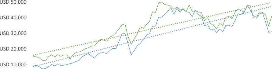
Balance of trade is an important indicator for economic activity, especially in countries that adopt open economy. Indonesia's balance of trade has been positive for the last two decades, as seen in Figure 1. A surplus in balance of trade can be considered good if both export and import are increasing, with a higher increase in export (Firdaus, 2020). The chart implies that Indonesia has been able to create healthy trade. This achievement certainly cannot be separated from the role of the government, particularly Bank Indonesia, which has the duty of maintaining the stability of Rupiah. Stability in this case is the stability against goods and services price and stability against other countries’ currencies (Bank Indonesia, 2020). The historical data shows that, although Indonesia's balance of trade is experiencing a surplus, the gap between exports and imports is narrowing. This fact raises the question of "Is the narrowing of Indonesia's export-import gap a sign that its trade performance is starting to decline?", despite the positive balance of trade. The linkage between exchange rate, inflation and the balance of trade, especially in countries that adopt an open economy system, has attracted considerable attention. However, there is only a few numbers of empirical evidences

regarding the causal relationship between, or dynamics of, the three macroeconomic

variables in the context of developing

countries (Yiheyis and Musila, 2018).

Figure 1. Indonesia’s Export-Import from 2001 to 2020

USD 60,000

USD 0

Export            Import            Linear (Export)            Linear (Import)

Source: International Monetary Fund (2020)

Many empirical studies on the effect of exchange rate on balance of trade have been conducted on various objects: bilateral and multilateral trades as well as multiple trading partner countries. Their findings also vary widely. Arize, Malindretos, and Igwe (2017) found a significant relationship in both short and long term between exchange rate and balance of trade. In the long term, exchange rate depreciation is able to improve balance of trade. Bahmani-Oskooee and Aftab (2018), using the ARDL model, found that exchange rate has a significant effect on balance of trade, in both short and long term. Similar results were found by Bahmani-Oskooee,

Bose, and Zhang (2017); Bahmani-Oskooee and Fariditavana (2015); Bahmani-Oskooee and Fariditavana (2016); Nusair (2016); Baek (2014); Firdaus et al. (2018); Bahmani-Oskooee and Aftab (2017); Aftab, Syed, and Katper (2017); Ginting (2013); and Arize (1994). Nevertheless, there are also studies that do not find a significant relationship between exchange rate and balance of trade. Rose (1991) found little evidence that exchange rate affects the balance of trade, indicating insignificance in some developing countries.

There have also been many empirical studies on the effect of exchange rate on inflation. Suhadak and Suciany (2020) found that exchange rate has a

significant effect on inflation in Indonesia through production costs. The depreciation of rupiah decreases the price of domestic goods for other countries, leading to increases in export demand and commodity prices. Kihangire and Mugyenyi (2005), using the ARDL model, also found that exchange rate has a significant effect on inflation. Similar results were found in other studies conducted in developing countries, e.g. Yiheyis (1997) and Klau (1998).

Inflation also affects balance of trade. When inflation rises, real exchange rate strengthens, so domestic goods become less competitive in world markets. This lowers exports and, subsequently, the balance of trade. Causality also appears in balance of trade-inflation relationship. When balance of trade increases, nominal exchange rate strengthens, and inflation weakens.

The depreciation of rupiah is a threat that must always be kept in check. The prolonged weakening of exchange rate endangers Indonesia’s real sector because its imports are dominated by raw and auxiliary materials and capital goods. The Ministry of Trade (2016) stated that

76.44% of Indonesia's imports are raw and auxiliary materials, 16.45% are capital goods, and 7.11% are consumer goods. This study attempts to analyze the dynamics of Indonesia’s exchange rate, inflation, and balance of trade against the world aggregate, which is represented by the country’s six major trading partners, namely China, Japan, Singapore, the United States, South Korea, and Malaysia. Based on the said background, this study seeks to identify the effects of exchange rates and inflation on balance of trade in Indonesia, the effects of balance of trade and inflation on exchange rate in Indonesia, the effects of balance of trade and exchange rates on inflation in Indonesia.

DATA

This study uses secondary data from Q1 of 2002 to Q4 of 2018. As all variables in this study cannot be obtained directly from secondary sources, initial calculations need to be made based on the components that make up the variables. The following are the data used in this study.

Table 1. Data, Symbol, and Source

No                       Data                        Symbol	Source
1   Indonesia’s Export                                           X 2   Indonesia’s Import                                         M	data.imf.org data.imf.org

No                       Data                        Symbol

Source

3  Indonesia – China Nominal Exchange Rate                  NER 4  Indonesia – Japan Nominal Exchange Rate                  NER 5   Indonesia – Singapore Nominal Exchange Rate               NER 6   Indonesia – the United States Nominal Exchange Rate         NER 7  Indonesia – South Korea Nominal Exchange Rate            NER 8   Indonesia – Malaysia Nominal Exchange Rate                NER 9   Consumer Price Index of Indonesia                          CPIIND 10  Consumer Price Index of China                             CPI 11  Consumer Price Index of Japan                             CPI 12  Consumer Price Index of Singapore                         CPI 13  Consumer Price Index of the US                            CPI 14  Consumer Price Index of South Korea                       CPI 15  Consumer Price Index of Malaysia                          CPI 16  The Weight of Indonesia – China Trade Activities            TAW 17  The Weight of Indonesia – Japan Trade Activities             TAW 18  The Weight of Indonesia – Singapore Trade Activities         TAW 19  The Weight of Indonesia – the US Trade Activities            TAW 20  The Weight of Indonesia - South Korea Trade Activities       TAW 21  The Weight of Indonesia – Malaysia Trade Activities          TAW 22  The Nominal GDP of Indonesia                        NGDPIND 23  The Nominal GDP of China                           NGDP 24  The Nominal GDP of Japan                           NGDP 25  The Nominal GDP of the US                          NGDP 26  The Nominal GDP of Singapore                         NGDP 27  The Nominal GDP of South Korea                      NGDP 28  The Nominal GDP of Malaysia                          NGDP 29  The Deflator GDP of Indonesia                           DGDPIND 30  The Deflator GDP of China                             DGDP 31  The Deflator GDP of Japan                              DGDP 32  The Deflator GDP of the US                            DGDP 33  The Deflator GDP of Singapore                           DGDP 34  The Deflator GDP of South Korea                         DGDP 35  The Deflator GDP of Malaysia                            DGDP 36  The Weight of Indonesia – China Export                     EW 37  The Weight of Indonesia – Japan Export                      EW 38  The Weight of Indonesia – the US Export                     EW 39  The Weight of Indonesia – Singapore Export                  EW 40  The Weight of Indonesia – South Korea Export                EW 41  The Weight of Indonesia – Malaysia Export                   EW 42  Indonesia’s Treasury Bill Rate                                 ITBR 43  London Interbank Offered Rate                            LIBOR

bi.go.id bi.go.id bi.go.id bi.go.id bi.go.id bi.go.id data.imf.org data.imf.org data.imf.org data.imf.org data.imf.org data.imf.org data.imf.org data.imf.org data.imf.org data.imf.org data.imf.org data.imf.org data.imf.org data.imf.org data.imf.org data.imf.org data.imf.org data.imf.org data.imf.org data.imf.org data.imf.org data.imf.org data.imf.org data.imf.org data.imf.org data.imf.org data.imf.org data.imf.org data.imf.org data.imf.org data.imf.org data.imf.org data.imf.org data.imf.org fred.stlouisfed.org

Source: Researcher (2021)

All data in Table 1 were then interest rate. This study uses two control calculated according to the variables used variables, namely relative macroeconomic in this study, namely balance of trade, real activities and relative interest rate; they effective exchange rate, inflation, relative were used to anticipate overestimates and macroeconomic activities, and relative

underestimates on the coefficients from       the          estimation          results.

	Table 2. Data, Symbol, and Position
No	Variable              Symbol                    Position
1 2 3 4 5	Real Effective Exchange Rate REER Dependent Variable and Independent Variable Inflation INF Dependent Variable and Independent Variable Balance of trade TB Dependent Variable and Independent Variable Real Macroeconomic Activities RMA Control Variable Relative Interest Rate RIR Control Variable

Source: Researcher (2021)

1)	Real Effective Exchange Rate (REER)        This method was chosen as a substitute for Jt1                               the Engle-Granger (1987) method, which REERt = ∑ TAWi x RERit requires that all variables must be CPIit                       integrated at the same level. One of the RERit = NERux    *                       6 CPIt                       advantages of ARDL is that it can be used by combining the variables in I (0) and I
2)	Inflation (INF)                                (1). To identify the long-term relationship, CPIInd-CPIInV                        1      1 .             1  .   1    1 ipjp =    t        t-1 xiqq%             bound testing needs to be done. Pesar, ‘        cpi‘-d Shin, and Smith (2001) explained that there are two sets of bound, namely the
3)	Balance of trade (TB) lower bound and the upper bound. When Xt- TB. t   Mt                                     we assume that all variables are at I(0), lower bound is generated. When we
4)	Real Macroeconomic Activities (RMA)       assume that all variables are at I(1), upper NGDP[nd                     bound is generated. Pesar, Shin, and Smith rMAt =---DGDPt------ (2001) suggested that this bound can be t  yn      NGDPit i=ι   iX DGDPit                  used when one part of the variables is at I(0) and the other part is at I(1). The
5)	Relative Interest Rate (RIR)                 maximum lag used to estimate the model RIRt = ITBRt — LIBORt                     is 4, equivalent to 1 year (four quarters). There are three models to be estimated

^{METHODOLOGIES}                        according to the research objectives; they

This study uses a time-series econometric      _{are Model 1, Model 2, and Model 3.}

model, namely Autoregressive Distributed

Lag (ARDL), developed by Pesar and Shin

(1999) and Pesar, Shin, and Smith (2001).

∆logREER_t = β₀

	nl
Model 1:	+ ∑ βikΔlogREERt-k
	k=1
n1	n2
∆logTBt = a0 + ∑ alkΔlogTBt-k	+ ∑ β2kΔlogTBt-k
k=ι	k=0
n2	n3
+ ∑ a2kΔlogREERt-k	+ ∑ β3kΔINFt-k
k=0	k=0
n3	n4
+ ∑ a3kΔINFt-k	+ ∑β4kΔlogRMAt-k
k=0	k=0
n4	n5
+ ∑a4kΔlogRMAt-k	+ ∑β3kΔRIRt-k
k=0	k=0
n5 + ∑a5kΔRIRt-k k=0	+ γ0logREERt-1 + γ1logTBt-1 + γ2INFt-1
+ λ0logTBt-1	+ γ3logRMAt-1 + γ4RIRt-1
+ λ1logREERt-1 + λ2INFt-1 + λ3logRMAt-1 + λ4RIRt-1	+ εt
+ μ	Model 3:
	n1
Model 2:	∆INFt = θ0 + ∑ θ1kΔINFt-k
	k=1
	n2
	+ ∑ θ2kΔlogTBt-k
	k=0
	n3
	+ ∑ θ3kΔlogREERt-k
	k=0
	n4
	+ ∑θ4kΔlogRMAt-k
	k=0
	n5
	+ ∑θ3kΔRIRt-k
	k=0

+ S^I N Ft-1 + δ1logTBt_-1

+ δ₂logREER_t-1

+ S₂IogRMAf-I + δ4RIRt_-1

^{+ v}t

The time-series method requires stationary data to avoid spurious regression. According to Gujarati (2009), the regression happens as the data only shows a trend; the high R² is the result of the trend, not the relationship between the dependent variable and the independent

variable. If the data is stationary, estimation using OLS can be done (Sugiyanto, 2004). There are several stationarity tests; they are chart analysis, correlogram test, and unit root test. This study uses unit root test and chart analysis (in addition to visual analysis). One of the commonly used methods is the Augmented Dickey-Fuller (ADF) test by adding the lag of the differentiation variable on the right side of the equation as a development from the previous unit

root test model, which can only be done if the time series data only follows the AR

pattern (1). In fact, in many cases, timeseries data contain higher AR elements

(Widarjono, 2017). The following is the formulation of the Augmented Dickey-

Fuller (ADF) test (Dickey and Fuller,

1979).

P

∆Y_t = γYt-ι + ∑βi∆Y_t-i₊ι + e_t l=2

P

^δy = «o ⁺ Y^γt-ι ⁺ ∑ βi^∆γt-i+1 ^{+ e}t

l=2

ΔYt = «o + «iT + yY_t-ι

P

+ ∑βiΔYt-i+ι + et i=2

Where: Y = observed variable; ΔYt = Yt – Yt-1 and T = time trend

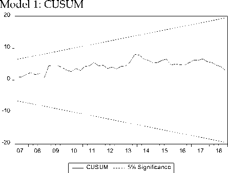
Following the model estimation, statistical diagnostic tests including Ramsey RESET (Regression Specification Error Test), CUSUM, CUSUMQ, Adjusted R², Normality, and Autocorrelation were performed.

RESULTS AND DISCUSSION

The results of the stationarity test using Augmented Dickey Fuller show that logINF is stationary at level with significance level of 1%, while logTB, logREER, logRMA, and RIR are stationary at first difference with significance levels of 1%, 1%, 5%, and 5%. Thus, based on the results of the unit root test, the data to be used is the combination of I(0) and I(1). RESET test results in Model 1 indicate that the probability value is higher than the significance level of 5%, so the null hypothesis is accepted. Therefore, it can be concluded that the model is appropriate. Model 2 also shows that the established model is also appropriate. Table 3 shows the summary of RESET test results. Model 3 shows that the probability value is lower than the significance level of 5%, so the null hypothesis is rejected. Hence, Model 3 is inaccurate. However, RESET test is only one of several model feasibility tests. There are still many other tests, such as

regression coefficient test, variable significance test through t test, R², Adjusted R², Durbin-Watson statistical value, MWD test etc. (Widarjono, 2017). If a measurement other than RESET is used, Model 3 is still feasible to use, even though the other two models are considered relatively better.

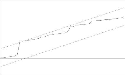
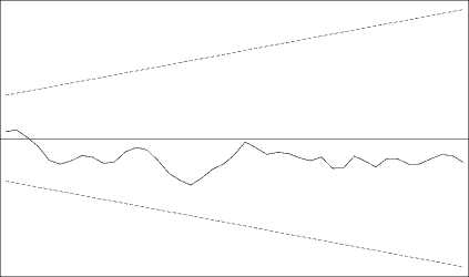
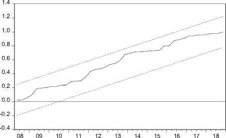
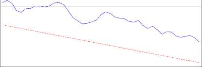
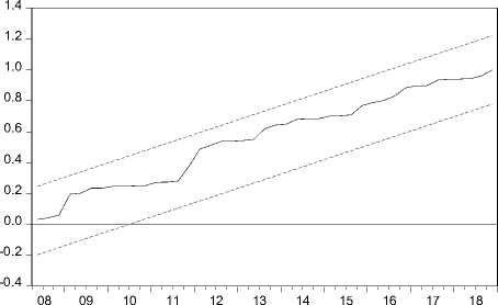
The results of the CUSUM and CUSUMQ tests for Model 1, 2, and 3 show the stability of the parameters, as shown in Figure 3. The recursive residual value is within the band at the critical line of 5%. The tests are indispensable for time-series data, which are often unstable due to structural changes in the study period. Moreover, the use of long period of time for research increases the likeliness of encountering structural changes such as crises, policy changes, natural disasters, non-natural disasters, etc.

Table 3. Descriptive Statistics, Unit Root Test Result, and Data Normality Test Result

Variable	Obs	Statistic Descriptive			SD	Augmented Dickey-Fuller			Saphiro-Wilk		Prob>z
		Mean	Max	Min		t-statistics	Prob	W	V	z
LogTB Level	68	0.2218	0.5440	-0.0541	0.1624	-1.8147	0.3704	0.9525	2.8510	2.274**	0.0111
First Difference LogREER Level	68	8.1787	8.4465	8.0276	0.0857	-9.2954*** -2.3891	0.0000 0.1487	0.9629	2.2290	1.740**	0.0409
First Difference INF Level	68	0.0157	0.1034	-0.0022	0.0144	-6.6184*** -7.6539***	0.0000 0.0000	0.7050	17.7350	6.243***	0.0000
First Difference LogRMA Level	68	-2.1128	-1.9336	-2.3363	0.1062	-8.3481*** -0.5176	0.0000 0.8798	0.9532	2.8130	2.245**	0.0123
First Difference RIR Level	68	0.0077	0.0277	-0.0137	0.0116	-3.2173** -2.2636	0.0239 0.1867	0.9615	2.3130	1.820**	0.0343
First Difference						-2.9824**	0.0419

Note: significant at 1%; ** significant at 5%; * significant at 10%

Null hypothesis: “variable has unit root”

max = maximum; min = minimum; SD = standard deviation

Source: IMF, World Bank, and Federal Reserve Bank of St. Louis (processed using E-Views 10)

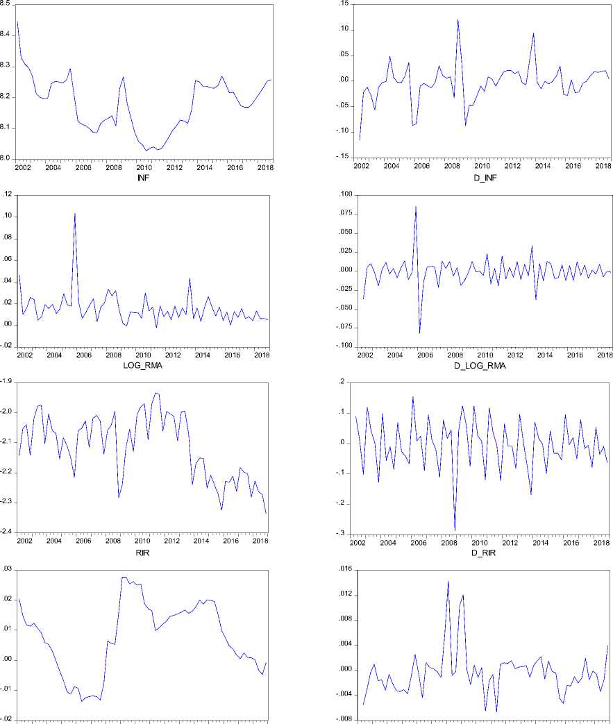
Figure 2. Charts of Variables at Level and First Difference

LOG_TB

.2

KΛ∕^vΛ

-.3

2002   2004   2006   2008   2010   2012   2014   2016   2018

D_LOG_TB

.1

.0

-.1

-.2

2002   2004   2006   2008   2010   2012   2014   2016   2018

LOG_REER

D_LOG_REER

2002   2004   2006   2008   2010   2012   2014   2016   2018

2002   2004   2006   2008   2010   2012   2014   2016   2018

Source: IMF, World Bank, and Federal Reserve Bank of St. Louis (processed using E-Views 10)

Gambar 3. CUSUM and CUSUMQ Test Results

Model 1: CUSUMQ

1.4

-0.4

1.2

1.0

0.8

0.6

0.4

0.2

0.0

-0.2

07    08    09    10    11    12    13    14    15    16    17    18

∣     CUSUM of Squares      5% Significance

Model 2: CUSUM

20

Model 2: CUSUMQ

-20

15

10

5

0

-5

-10

-15

18

08    09    10    11     12     13    14    15    16    17

CUSUM of Squares     5% Significance

I--- CUSUM      5% Significance1

Model 3: CUSUM

20

Model 3: CUSUMQ

15

10

5

0

-20

-5

-10

-15

08    09    10    11     12    13    14    15    16    17    18

CUSUM of Squares     5% Significance

CUSUM     5% Significance

Source: IMF, World Bank, and Federal Reserve Bank of St. Louis (processed using E-Views 10)

The ability of the independent variables in explaining the dependent variable is relatively better in Model 1 and Model 2 than in Model 3. The results of the normality test performed on all models show a probability value that is higher than the significance level of 5%, so the null hypothesis is accepted, which means that the residual in all model is normally

distributed. Model 1 and 3 do not contain autocorrelation, but autocorrelation is found in Model 2. Hence, improvements need to be made for Model 2, namely using the Newey-West method, which was popularized by Newey and West (1987). The results of estimation for Model 2 in Table 3 show that the model is autocorrelation-free.

	Table 4. Bound Test Results
Significance Level	Model 1             Model 2            Model 3 Lower  Upper Dependent Variable:   Dependent Variable:   Dependent Variable: Bound  Bound ΔlogTBt             ΔlogREERt             ΔINFt F-statistic                 F-statistic                F-statistic
10% 5% 1%	2.2      3.09 2.56     3.49            2.8997 14.3603                 6.2626 3.29     4.37

Source: IMF, World Bank, and Federal Reserve Bank of St. Louis (processed using E-Views 10)

In order to identify the long-term relationship, a cointegration test is required. The results of the bound test show that the F-statistical value of Model 2 and Model 3 is greater than the upper bound of I(1) at the significance levels of 10%, 5%, and 1%, which means that there is a cointegration or long-term relationship between variables in Model 2 and Model 3. The F-statistic value of Model 1 is below the upper bound of I(1) but above the lower bound of I(0). According to Yiheyis and Musila (2018), if the F-statistic value is

below the lower limit of I(0), cointegration does not occur. Because the F-statistic value of Model 1 is still above I(0), the cointegration appears in Model 1 even though it is not strong enough as the value is between the upper and lower bound. Considering that the data is the combination of level and first difference, the two bound values can be used when one part of the data is at I(0) and the other part of the data is at I(1) (Pesar, Shin, and Smith, 2001).

Table 5. Result of Short-Term Estimation

Model 1

Model 2

Model 3

Dependent Variable:    Dependent Variable:    Dependent Variable:

Explanatory Variables         _{ΔlogTBt              ΔlogREERt               ΔINFt}

	coefficient	t-statistic	coefficient	t-statistic	coefficient	t-statistic
ΔlogTBt	-	-	-0.0728	-1.9612***	-0.0206	-0.8208
ΔlogTBt-1	-0.2953	-1.8995*	-0.0702	-2.0607**	-0.0660	-2.5237**
ΔlogTBt-2	-0.2807	-1.8752*	0.0776	2.5566**	-	-
ΔlogTBt-3	-0.3763	-2.6233**	-	-	-	-
ΔlogTBt-4	-	-	-	-	-	-
ΔlogREERt	-0.8206	-2.4820**	-	-	-0.5726	-6.0963***
ΔlogREERt-1	0.2844	0.9644	0.4535	4.4390***	-0.3219	-3.3549***
ΔlogREERt-2	-0.8365	-2.7204***	0.0617	0.5472	-0.1612	-1.7494*
ΔlogREERt-3	0.3508	1.3681	-0.0710	-0.5551	-0.2597	-3.3264***
ΔlogREERt-4	-	-	0.4778	6.1378***	-	-
ΔINFt	-0.0154	-0.0246	-0.8096	-7.2107***	-	-
ΔINFt-1	-2.5960	-2.4888**	-0.2578	-1.4034	0.3327	1.6056
ΔINFt-2	-2.2853	-2.6563**	-0.0288	-0.1665	0.3833	2.3994**
ΔINFt-3	-0.9008	-1.5769	-0.4180	-5.9027***	0.1391	1.3248
ΔINFt-4	-	-	-0.2105	-2.3826**	-	-
ΔlogRMAt	-	-	-0.5684	-13.923***	-0.2989	-4.3603***
ΔlogRMAt-1	-	-	0.0984	2.6590**	-0.3456	-4.7209***
ΔlogRMAt-2	-	-	0.1392	3.6467***	-0.2033	-2.8536***
ΔlogRMAt-3	-	-	-0.0468	-1.1015	-0.2384	-3.4938***
ΔlogRMAt-4	-	-	0.4811	8.5999***	-	-
ΔRIRt	-	-	0.6716	1.4208	0.3612	0.7377
ΔRIRt-1	-	-	-0.0655	-0.0908	1.1143	2.1049**
ΔRIRt-2	-	-	-1.2860	-1.9759*	-	-
ΔRIRt-3	-	-	-	-	-	-
ΔRIRt-4	-	-	-	-	-	-
#obs	64		64		64
R2	0.8827		0.9819		0.6436
Adjusted R2	0.8427		0.9735		0.4779
F-statistic	22.10***		116.94***		3.8840***
Autocorrelation (prob)	0.1275		0.0017		0.1728
Normality (prob)	0.2866		0.6740		0.0588
Ramsey RESET (prob)	0.9565		0.2773		0.0000

note: *** significant at 1%; ** significant at 5%; * significant at 10%

Source: IMF, World Bank, and Federal Reserve Bank of St. Louis (processed using E-Views 10)

Table 6. Result of Long-Term Estimation

Explanatory Variables	Model 1 Dependent Variable: ΔlogTBt		Model 2 Dependent Variable: ΔlogREERt		Model 3 Dependent Variable: ΔINFt
	coefficient	t-statistic	coefficient	t-statistic	coefficient	t-statistic
logTBt	-	-	-0.8403	-1.6310	-0.0327	-3.1676***
logREERt	0.0269	0.0217	-	-	0.0035	0.1798
INFt	28.5202	1.3798	-22.1363	-1.8314*	-	-
logRMAt	-0.7456	-0.5172	1.3294	1.3674	0.0681	4.3317***
RIRt	5.5373	0.6908	-8.7262	-1.8354*	-0.3876	-5.6183***
C	-2.2002	-0.2661	11.4357	4.9345***	0.1370	0.8734

note: *** significant at 1%; ** significant at 5%; * significant at 10%

Source: IMF, World Bank, and Federal Reserve Bank of St. Louis (processed using E-Views 10)

Depreciation of real effective exchange rate in the short term has a significant negative effect on the balance of trade at lag 0 and lag 2, while at lag 1 and lag 3, it does not significantly affect the balance of trade, but the correlation is positive. The estimation results in this study indicate that, when real exchange rate depreciates, the balance of trade immediately decreases. In the following quarter, the balance of trade improved although not significantly. The depreciation of real exchange rate makes the prices of domestic goods relatively lower than those of foreign goods, so export demand increases followed by balance of trade (Mankiw, 2016). This result follows the J-Curve theory, in which the balance of trade of a country immediately deteriorates after depreciation and will improve several months later (Krugman, Obstfeld, and

Melitz, 2018). According to Nusair (2016), there are two empirical definitions regarding the J-Curve. The first is the definition by Bahmani-Oskooee (1985) that J-Curve occurs when the exchange rate coefficient is negative at the lowest lag followed by a positive coefficient value at the highest lag. The second is the definition by Rose and Yellen (1989) that J-Curve occurs when the exchange rate coefficient is negative or insignificant in the short term but positive and significant in the long term. The results of this study’s estimation are more inclined to the definition proposed by Bahmani-Oskooee (1985) than to the definition by Rose and Yellen (1989).

Measured in domestic currency, balance of trade might fall sharply after the depreciation as some import and export orders were placed in the preceding months. The main impact of

depreciation will increase the value of previously agreed imports measured in the domestic currency. The negative and significant relationship between real effective exchange rate and balance of trade in the short term is also caused by raw materials and capital goods that dominate Indonesia's imports, so the demand is inelastic. These types of goods must still be imported to ensure the smooth running of domestic production activities to avoid inflation and unemployment. The estimation results also show that in the long run the real effective exchange rate does not significantly influence the balance of trade, but the correlation is positive. This shows that depreciation in the long run could improve the balance of trade. Theoretically, the coefficient has shown the right direction even though the value is insignificant.

Inflation in the short term has a significant negative effect on balance of trade at lag 1 and lag 2, but it does not significantly affect balance of trade at lag 0 and lag 3, yet the correlation is negative. This study’s estimation results indicate that, when inflation increases, the balance of trade decreases. Inflation can affect balance of trade through real exchange rate channel. At a certain nominal (unchanged) exchange rate, an increase in inflation will lead to an increase in real

exchange rate, so foreign goods will become relatively cheaper, and imports will increase. Nevertheless, the strengthening of real exchange rate makes domestic goods uncompetitive. In other words, domestic goods become more expensive abroad, so export demand falls, and balance of trade worsens. In the long run, the estimation results show that inflation does not have any significant effect on balance of trade because the nominal exchange rate can neutralize changes in the real exchange rate caused by changes in inflation. Purchasing power parity theory states that exchange rate between two currencies of two countries is the same as the price level ratio in the two countries (Krugman, 2018). The domestic purchasing power of a country's currency is fully reflected in the price level prevailing in that country itself. Thus, the purchasing power parity theory states that a decrease in the purchasing power of a domestic currency (indicated by an increase in domestic prices) will be accompanied by a proportional depreciation of the currency in the foreign exchange market. Conversely, an increase in the purchasing power of the domestic currency will be followed by a proportional appreciation of the currency. The nominal exchange rate in the long run can change and adjust accordingly. If inflation increases, the real exchange rate

that is supposed to be appreciated becomes neutralized due to depreciation in the nominal exchange rate based on the purchasing power parity theory, so inflation does not affect balance of trade. In the long run, relative macroeconomic activity and relative interest rate do not have any significant effect on balance of trade.

Balance of trade in the short-term has a significant negative effect on real effective exchange rate at lag 0, lag 1, and lag 2. The estimation results of this study show that, when the balance of trade increases, the real exchange rate appreciates, and when the balance of trade falls, the real exchange rate depreciates. This can occur through nominal exchange rate channel. When the balance of trade strengthens (due to an increase in exports), the demand for domestic currency will increase because overseas buyers have to convert their currency into domestic currency. As a result, the nominal exchange rate appreciates, followed by the real exchange rate. An increase in the balance of trade (due to lower imports) reduces the demand for domestic currency, so the nominal exchange rate depreciates followed by the real exchange rate. In the long run, the balance of trade does not have any significant effect on real effective exchange rate, but the correlation is negative.

Inflation in the short term has a significant negative effect on real effective exchange rate at lag 0, lag 3, and lag 4, but it does not have any significant effect at lag 1 and lag 2. This study’s estimation indicates that, when inflation increases, the real exchange rate will be appreciated, and when inflation decreases, the exchange rate will be depreciated. This is because, when the price of domestic goods rises, foreign countries will get fewer domestic goods than before. In other words, the real exchange rate improves. In the long run, inflation has a significant negative effect on real effective exchange rate.

Relative macroeconomic activities in the short term have a significant negative effect on real effective exchange rate at lag 0; while at lag 1, lag 2, and lag 4, the effect is significant and positive. Relative macroeconomic activities do not significantly affect real effective exchange rate at lag 3. Based on Table 5, the sum of the coefficient values for all lags is still positive, so in the short term, the correlation between relative macroeconomic activities and real effective exchange rate is positive. In other words, when the relative macroeconomic activities increase, as measured by Indonesia's GDP against other countries’ GDP, real exchange rate depreciates. This occurs over a long course. An increase in

relative macroeconomic activities increases the demand for imports because domestic production still requires raw materials and capital goods from abroad. As a result, the balance of trade weakens, and real exchange rate depreciates. A vicious circle is formed from these variables. After the depreciation of real exchange rate, exports increase, and relative macroeconomic activities also increase, and so on. In the long term, relative macroeconomic activities have no significant effect on real effective exchange rate, but the correlation is positive. This is caused by technological advancement in the long run, as stated by Solow's (1956) long-term growth theory. In the long term, technological advancement can create new production techniques. However, there is still a possibility that the raw materials and capital goods still have to be imported, but such technological changes can at least reduce the imports. Hence, the increase in relative macroeconomic activities will not affect the real effective exchange rate in the long run.

Relative interest rate, in the short run, has a significant negative effect on real effective exchange rate at lag 2, while its effects at lag 0 and lag 1 are insignificant. In the long term, relative interest rate also has a significant negative effect. The estimation results in that, when the relative interest rate increases, the real

effective exchange rate will be appreciated because the higher the relative domestic interest rate against the foreign interest rate, the higher the demand for domestic currency. Thus, nominal exchange rate appreciates, followed by an increase in real exchange rate.

Balance of trade in the short term has a significant negative effect on inflation at lag 1, while at lag 0 it has no significant effect. In the long term, it also has a significant negative effect on inflation. The estimation results of this study indicate that, when the balance of trade improves, inflation decreases. When the balance of trade improves (due to increased exports), the nominal exchange rate appreciates and reduces inflation. Likewise, when the balance of trade improves due to decreased imports, domestic demand for foreign currencies also decreases so that nominal exchange rate improves and subsequently reduces inflation.

Real effective exchange rate in the short term has a significant negative effect on inflation at lag 0, lag 1, lag 2, and lag 3. The estimation results of this study indicate that, when real exchange rate depreciates, inflation decreases because, when the exchange rate depreciates, exports increases. In other words, balance of trade improves. What will happen next is that nominal exchange rate appreciates

and reduces inflation. In the long term, real effective exchange rate does not have any significant effect on inflation.

Relative macroeconomic activities have a significant negative effect on inflation at lag 0, lag 1, lag 2, and lag 3. The estimation results of this study indicate that an increase in relative macroeconomic activity will increase the domestic aggregate supply, so inflation decreases because demand in the short term cannot follow the aggregate supply unless expansionary fiscal policy, expansionary monetary policy, or changes in preferences are made and public expectations are raised. However, in the long term, the increase in relative macroeconomic activities has a positive significant effect on inflation. The relative interest rate has a significant positive effect on inflation at lag 1, while at lag 0 it has no significant effect. In the long term, relative interest rate has a significant negative effect on inflation. The higher the relative interest rate, the lower the inflation. This occurs because high interest rates can reduce aggregate demand and further reduce prices for goods and services in general.

CONCLUSION AND RECOMMENDATION

The findings of this study lead to conclusions that dynamics occur between

exchange rate, inflation, and balance of trade in Indonesia and that, in the short term, causality appears between exchange rate and balance of trade, exchange rate and inflation, and balance of trade and inflation. The estimation results also show the occurrence of J-Curve phenomenon in Indonesia; that is when exchange rate depreciates, balance of trade will begin to improve in the second and fourth quarters. Given that most of Indonesia's imports are raw materials and capital goods, the depreciation of exchange rate will adversely affect domestic production activities. Therefore, Bank Indonesia must be able to maintain exchange rate stability better. In addition, as inflation has a negative effect on balance of trade through real exchange rate channel, Bank Indonesia must be able to improve their performance in maintaining price stability for domestic goods so that they remain competitive in the world market.

REFERENCE

Aftab, M., Syed, K.B.S., & Katper, N.A. 2017. Exchange-Rate Volatility and Malaysian-Thai Bilateral Industry Trade Flows. Journal of Economic Studies Vol. 44 No. 1 pp. 99-114.

Arize, A.C. 1994. Cointegrating Test of a Long-Run Relation Between the Real Effective Exchange Rate and the Balance of trade. International Economic Journal Vol. 8 No.3, pp 1-9

Arize, A.C., Malindretos, J., & Igwe, E.U. 2017. Do Exchange Rate Changes Improve the Balance of trade: An Asymmetric           Nonlinear

Cointegration          Approach.

International Review of Economics and Finance Vol. 49 pp. 313-326.

Baek, J. 2014. Exchange Rate Effects on Korea–US Bilateral Trade: A New Look. Research in Economics Vol. 68 pp. 214-221.

Bahmani-Oskooee, M. 1985. Devaluation and the J-Curve: Some Evidence from LDCs. Review of Economics and Statistics Vol. 67 No.3, pp. 500-504.

Bahmani-Oskooee, M., & Aftab, M. 2018. Asymmetric Effects of Exchange Rate Changes on The Malaysia-China Commodity Trade. Economic Systems Vol. 42 pp. 470-486.

Bahmani-Oskooee, M., Bose, N., & Zhang, Y.       2017.       Asymmetric

Cointegration, Nonlinear ARDL and the J-curve:  A Bilateral

Analysis of China and its 21 Trading Partners. Emerging Markets Finance and Trade Vol. 54 No. 13 pp. 3131-3151.

Bahmani-Oskooee, M., & Aftab, M. 2017. On the Asymmetric Effects of Exchange Rate Volatility on Trade Flows: New Evidence from US-Malaysia Trade at the Industry Level. Economic Modelling Vol. 63 pp. 86-103.

Bahmani-Oskooee, M., & Fariditavana, H. 2015. Nonlinear ARDL Approach, Asymmetric Effects and The J-Curve. Journal of Economic Studies Vol. 42 No. 3 pp. 519-530.

Bahmani-Oskooee, M., & Fariditavana, H. 2016. Nonlinear ARDL Approach and The J-Curve Phenomenon. Springer Science+Business Media New York pp. 51-70.

Bank Indonesia. 2020. Status dan Kedudukan     Bank     Indonesia.

https://www.bi.go.id/id/tentang-bi/profil/Default.aspx. Februari 2021.

Dickey, D.A.,  & Fuller, W.A. 1979.

Distribution of the Estimators for Autoregressive Time Series with a Unit Root. Journal of the American Statistical Association, Vol. 74, pp 427-43.

Engle, R.F., & Granger, C.W.J. 1987. CoIntegration and Error Correction: Representation, Estimation, and Testing. Econometrica, Vol. 55 No.2, pp. 251-276.

Firdaus, A.H. 2020. Surplus Neraca Perdagangan Indonesia Masih Belum Sehat.

https://www.beritasatu.com/eko nomi/699069/surplus-neraca-perdagangan-indonesia-masih-belum-sehat. Februari 2021.

Firdaus, M.,Holis, A.,Amaliah, S., Fazri, M., & Sangadji, M. 2018. Dampak Pergerakan Nilai Tukar Rupiah Terhadap Aktivitas Ekspor dan Impor Nasional. Indonesia Exim Bank dan FEM IPB.

Ginting, A.M. 2013. Pengaruh Nilai Tukar Terhadap Ekspor Indonesia. Buletin Ilmiah Litbang Perdagangan Vol.7 No.1

Gujarati, D.N., & Porter, D.C. 2009. Basic Econometrics. 5^th Edition. McGraw-

Hill/Irwin. United States of America.

IMF. 2000. Globalization:   Threat or

Opportunity?.

https://www.imf.org/external/np /exr/ib/2000/041200to.htm.

Februari 2021.

IMF. 2002. Globalization: A Framework for IMF                  Involvement.

https://www.imf.org/external/np /exr/ib/2002/031502.htm.

Februari 2021.

IMF. 2020. International Financial Statistics, External Sector Selected Indicators – Indonesia.

https://data.imf.org/regular.aspx? key=61545851. Januari 2021.

Kementerian Perdagangan. 2016. Kajian Peran Kebijakan Impor Dalam Rangka Mendukung Industri Manufaktur: Studi Kasus Industri Kimia, Tekstil, dan Produk Tekstil, dan Elektronik. Pusat Pengkajian Perdagangan Luar Negeri, Badan Pengkajian dan Pengembangan Perdagangan          Kementerian

Perdagangan Republik Indonesia.

Kihangire, D., & Mugyenyi, A. 2005. Is Inflation Always and Everywhere a Non-Monetary     Phenomenon:

Evidence from Uganda. Bank of Uganda Staff Papers.

Klau, M. 1998. Exchange Rate Regime and Inflation and Output in SubSaharan African Countries. Working  Paper 53,  Banking for

International Settlements.

Krugman, P.R., Obstfeld, M., & Melitz, M.J. 2018. International Economics: Theory and Policy. 11ed. London. Pearson.

Mankiw, N.G. 2016. Macroeconomics. 9ed. New York. Worth.

Newey, W., & West, K. 1987. A Simple Positive             Semi-Definite,

Heteroskedasticity            and

Autocorrelation         Consisten

Covariance Matrix. Econometrica, Vol. 55, pp. 703-708.

Nusair, S.A. 2016. The J-Curve Phenomenon    in    European

Transition Economies: A Nonlinear ARDL Approach. International Review of Applied Economics Vol. 31 No. 1 pp. 1-27.

Pesaran, H.,  & Shin, Y. 1999. An

Autoregressive Distributed Lag Modelling     Approach     to

Cointegration.  Econometrics  and

Economic Theory in the 20^th Century: The Ragnar Frisch Centennial Symposium.

Pesaran, M.H., Shin, Y., & Smith, R. 2001. Bounds Testing Approaches to the Analysis of Level Relationship. Journal of Applied Econometrics, Vol. 16 No.3, pp. 289-326.

Rose, A.K. 1991. The Role of Exchange Rates in a Popular Model of International Trade:  Does the

Marshall-Lerner Condition Hold?. Journal of International Economics Vol. 30 No. ¾ pp. 301-316

Rose, A.K., & Yellen.,J.L. 1989. “Is There a J-Curve?”  Journal of Monetary

Economics Vol.24 No. 1, pp. 53-68.

Solow, R.M. 1956. A Contribution to the Theory of Economic Growth. Quarterly Journal of Economics Vol. 70 No.1, pp. 56-94.

Sugiyanto, F.X. 2004. Faktor-faktor yang Mempengaruhi Perilaku Kurs Rupiah Terhadap Dolar the United States di Indonesia Tahun 19861997: Sintesis Pendekatan Moneter dan    Pendekatan    Portofolio.

Disertasi, Sekolah Pasca Sarjana Ilmu    Ekonomi,    Universitas

Airlangga.

Suhadak & Suciany, A.D. 2020. The Influence of Exchange Rates on Inflation, Interest Rates and the Composite Stock Price Index: Indonesia 2015-2018. Australasian

Accounting, Business and Finance Journal Vol 14 Issue 1.

Widarjono, A. 2017. Ekonometrika. Edisi ke-4. UPP STIM YKPN. Yogyakarta.

Yiheyis, Z. 1997. Output Growth and Inflation      Adjustment      to

Devaluation  Episodes in  Sub

Saharan Africa. Canadian Journal of Development Studies Vol.18 No.1, pp.93-117.

Yiheyis, Z.,  & Jacob, M. 2018. The

Dynamics of Inflation, Exchange Rates and the Balance of trade in a Small Economy: The Case of Uganda. International Journal of Development Issues Vol. 17 Issue: 2, pp.246-264.

294