Volatilitas inflasi sebagai fenomena kombinasi moneter-fiskal di Indonesia

ISSN : 2301-8968

Vol. 14 No.2, Agustus 2021

EKONOMI

KUANTITATIF

TERAPAN

Volume 14

JEKT

Nomor 2

ISSN 2301-8968

Denpasar Agustus 2021

Halaman

243-431

Balinese Indigenous Knowledge about Water : A Way to Achieve Water Sustainability

Amrita Nugraheni Sarawaty, I Wayan Gita Kesuma, I Gusti Wayan Murjana Yasa

Planning Consistency and the Political Budget Cycle in Indonesia Farina Rahmawati, Khoirunurrofik Khoirunurrofik

PROVINCE Analysis of Financial Institutions Credit Impact on MSE Income in Bali Province Ksama Putra, Ni Putu Wiwin Setyari

The Dynamics of Credit Procyclicality and Stability of Macroeconomics in Indonesia Ni Putu Nina Eka Lestari, Made Kembar Sri Budhi, I Ketut Sudama, Ni Nyoman Reni Suasih, I Nyoman taun

The The Impact of COVID-19 on FinTech Lending in Indonesia: Evidence From Interrupted Time Series Analysis

Abdul Khaliq

The Dynamics of Exchange Rate, Inflation, and Trade Balance in Indonesia Yon Widiyono, David Kaluge, Nayaka Artha Wicesa

Volatilitas inflasi sebagai fenomena kombinasi moneter-fiskal di Indonesia Eli Marnia Henira, Raja Masbar, Chenny Seftarita

The Analysis of Willingness to Pay (WTP) Visitors to The Development of Rafting Toutism in Serayu Watershed

Nobel Sudrajad, Waridin, Jaka Aminata, Indah Susilowati

Relatiomships Between Characteristic of Local Government and Website Based Financial Gabriela Amanda Widyastuti, Dena Natalia Damayanti, Marwata

The Relationship Among Economic Structure, Sectoral Workforce, and Community Welfare in Bali Province I Nyoman Mahendrayasa

pISSN : 2301 – 8968

JEKT ♦ 14 [2] : 305-324

eISSN : 2303 – 0186

Volatilitas inflasi sebagai fenomena kombinasi moneter-fiskal di Indonesia Inflation volatility as a phenomenon monetary-fiscal combination in Indonesia Eli Marnia Henira

Raja Masbar

Chenny Seftarita

Universitas Syiah Kuala

Abstrak

Inflasi umumnya dipandang sebagai fenomena moneter yang pengendaliannya efektif melalui pengelolaan jumlah uang beredar, suku bunga, dan nilai tukar. Pendapat lain memandang inflasi sebagai fenomena fiskal yang dikendalikan melalui efektifitas penerimaan pajak dan pengeluaran negara serta menghindari defisit anggaran yang memicu kenaikan utang luar negeri pemerintah. Penelitian ini bertujuan untuk menguji dan menganalisis volatilitas inflasi sebagai fenomena kombinasi moneter-fiskal di Indonesia. Analisis dilakukan secara deskriptif dan kuantitatif melalui Model Autoregressive Distributed Lag (ARDL) menggunakan data sekunder time series mulai kuartal 1 tahun 2009 hingga kuartal 2 tahun 2020. Hasil penelitian menunjukkan dominasi pengaruh positif suku bunga dari sisi moneter dan utang luar negeri dari sisi fiskal, serta belum efektifnya peran penerimaan pajak dalam menurunkan inflasi di Indonesia. Bank Indonesia perlu mengefektifkan kebijakan terkait pengelolaan suku bunga dalam mengatur jumlah uang beredar. Pemerintah perlu mengupayakan peningkatan efektifitas penerimaan pajak dan belanja negara untuk minimalisir utang luar negerinya.

Kata kunci: Inflasi, Moneter, Fiskal, Model ARDL, Indonesia.

JEL classification: C32, E31, E52, E62.

Abstract

Inflation is generally seen as a monetary phenomenon whose effective control is through the management of the money supply, interest rates, and exchange rates. Another opinion views inflation as a fiscal phenomenon that is controlled through the effectiveness of tax revenues and state expenditures and avoiding a budget deficit that triggers an increase in government external debt. This study aims to examine and analyze the volatility of inflation as a phenomenon monetary-fiscal combination in Indonesia. The analysis was carried out descriptively and quantitatively through the Autoregressive Distributed Lag (ARDL) Model using secondary time series data from the 1st quarter of 2009 to the 2nd quarter of 2020. The results showed the dominance of the positive influence of interest rates from the monetary side and foreign debt from the fiscal side, as well as the ineffective role of tax revenue in reducing inflation in Indonesia. Bank Indonesia needs to streamline policies related to interest rate management in regulating the money supply. The government needs to make efforts to increase the effectiveness of tax revenues and state spending to minimize its foreign debt.

Keywords: Inflation, Monetary, Fiscal, ARDL Model, Indonesia.

JEL classification: C32, E31, E52, E62.

1. Introduction

Inflation volatility is a condition of inflation that is unstable, tends to vary and is difficult to estimate. Inflation instability will cause uncertaintyin decision-making to investand produce (for producers) andconsume (for consumers). This is due to the close link between inflation uncertainty and the cost of production and the price of the resulting commodity. In addition, the Granger causality test conducted by Jiranyakul and Opiela (2010) showed that rising inflation will increase inflation uncertainty and rising inflation uncertainty will raise inflation rates in Indonesia, Malaysia, the Philippines, Singapore, and Thailand.

Inflation volatility can lead to excessive inflation expectations. Where inflation expectations tend to increase along with the acceleration of inflation (Feldkircher and Siklos, 2019). This happens because inflation expectations play an important role in the pricing process in the market (Soybilgen and Yazgan, 2017; Binder, 2018; Berge, 2018; Hammoudeh and Reboredo, 2018) .

Expectations arise because of information. Household inflation expectations are more responsive to inflation news (Baqaee, 2019) and have a central role in the implementation of monetary policy (Das, Lahiri and Zhao, 2019). Information about inflation in the past plays a role in current inflation expectations and volatility. Market risks will increase due to very low or high inflation expectations and not react to moderate or stable inflation

expectations (Orlowski and Soper, 2019). Price stability will significantly reduce inflation expectations (Rumler and Valderrama, 2020).

The idea of inflation is generally understood as a monetary phenomenon as seen from nobel laureate Milton Friedman's statement when he lectured at the University of London on 16 September 1970 that "inflation is always and everywhere also a monetary phenomenon" (Hossain, 2010: 142). The basis is the theory of monetarists who argue that money growth is the main source of inflation (Jahan and Papageorgiou, 2014).

The empirical results of Jongwanich and Park (2009) show that Asian inflation comes mostly from within the country due to excess aggregate demand and inflation expectations. In this regard, he argues that monetary policy will remain the best tool in overcoming inflation in Asia. The policy is related to controlling the money supply, interest rates,and exchange rates/ exchange rates.

In addition to the view of inflation as a monetaryphenomenon, there has long been growing thinking related to inflation as a fiscal phenomenon. This thinking is based on The Fiscal Theory of The Price Level. This theory states that inflation (pricelevel) has no direct relationship with monetary policy, but is influenced by fiscal conditions in the form of government spending plans including to pay its debtsand receipts from the sector pertax (Hervino, 2011). Thus it was concluded that inflation is determined by the budgetary policies

of fiscal authorities (Carlstrom and Fuerst, 2000).

While Tutino and Zarazaga (2014) arguethat fiscal policy is just as important andsometimes more important than monetary policy in themenentukan tingkat Price and inflationdynamics. According to this thinking, inflation control is not enough through monetary policy, but should also be done through fiscal policy. The policy is related to the effectiveness of state spending and tax revenues and avoids the occurrence of budget deficits that trigger increases in government debt.

Research on inflation in Indonesia related to its status as a fiscal or monetary phenomenon was conducted by Hervino (2011). He looked at the fiscal side of the government's foreign debt variable while the monetary side was reviewed from the variable amount of money supply. The results showed the money supply and foreign debt in the short term had a negative impact on Indonesia's inflation. However, the opposite happens in the long run, where the money supply and foreign debt positively affect the volatility of inflation in the country. So he concluded that the monetary and fiscal side in the long term will affect the volatility of inflation in Indonesia. However, after the 1997 economic crisis, the monetary side was more dominant in influencing inflation volatility than the fiscal side. This is evidenced by the high coefficient of the money supply (0.031946)

compared to the coefficient of foreign debt (0.000791).

Azhar et al. (2019) also found theomnation ofmonetary phenomena over long-term regional inflation in West Sumatra. In more detail, the results showed that the money supply (M2) negatively did notaffect it in the short term and was positively significant in the long term. Interest rates arepositively significant in the short and longterm. Government spending has asignificant negative effect in the long term and negative is not significant in the short term. In the short and long term, local taxes have an insignificant negative influence on inflation in West Sumatra.

There is a lot of research on inflation that is reviewed from the monetary aspect, but there are still limited researchers who examine inflation from the fiscal aspect. One of them is Surjaningsih et al. (2012) which examines the impact of fiscal policy on output and inflation. His research is based on the fiscal theory of the price level, where fiscal policy plays an important role in pricing through budget constraints related to debt policy, spending and taxation. Among the results of his research found that increases in government spending led to a decrease in inflation, while increased taxes led to an increase in inflation. The effect of debt policy and monetary factors on inflation was not discussed in the study.

Related to government debt, Trisdian et al. (2015) found that local government debt does not have asignificant influence on the regional inflation ratein Indonesia. Nevertheless, fiscal transparency has a strong negative effect on inflation (Montes and da Cunha Lima, 2018).

This difference of thought is behind researchers to study the volatility ofinflation, especially in Indonesia. During the period of Q1 of 2009 to Q2 of 2020, the highest inflation rate in Indonesia ever reached 8.4 percent and the lowest 1.96 percent with an average value of 4.65 percent. The highest inflation occurred in the third quarter of 2013. This was triggered by an increase of 18.92 percent in the USD exchange rate and 22.41 percent in government spending compared to the same quarter a year earlier. Inflation remains high although at the same time the government is already trying to lower it by increasing tax revenue growth by 13.2 percent and increasing interest rates from 6 percent in the previous period to 7.25 percent.

The lowest inflation occurred in the second quarter of 2020, when the Covid-19 outbreak began to hit Indonesia. The decrease in inflation occurred due to a decrease in the money supply of 46.71 trillion rupiah and an increase in tax revenues of 65.12 trillion rupiah compared to the previous period. The increase in tax revenue was triggered by an increase in government spending of 164.12 trillion rupiah or an increase of 36.28 percent from the previous quarter. In addition, the rupiah exchange rate

against the US dollar also strengthened from 16,310 rupiah to 14,265 rupiah.

Based on differences in theoretical views and data, the question arises, is inflation volatility in Indonesia a phenomenon of monetary-fiscal combination? In connection with that, the study aims to test and analyze inflation volatility as a phenomenon of monetary-fiscal combination in Indonesia.

The novelty of this study lies in the completeness of the variables used in assessing inflation volatility as a phenomenon of monetary-fiscal combination in Indonesia. Monetary phenomena are seen from the factor of the money supply, interest rates, and exchange rates. While the fiscal phenomenon is seen from the factors of tax revenue, state spending, and foreign debt carried out by the government to cover the budget deficit. Thus, the phenomenon of monetary-fiscal combination is seen from the interaction of all these factors in influencing inflation volatility in Indonesia.

• 1.    Data

This study uses secondary data in the form of time series starting from Q1 of 2009 to Q2of2020 obtained from Bank Indonesia (BI) and the Ministry of Finance. The objects of his research are inflasi, the amount of money,interest rates, exchange rates, taxrevenues, government spending,and foreign debt. The analysis was conducted descriptively and quantitatively using the Autoregressive Distributed Lag (ARDL)

Model with the help of the Eviews 10 application.

As a dependent variable in this study, inflation is the percentage change in the Consumer Price Index (CPI) in the quarter concerned compared to the cpi of the same quarter in the previous year with a unit of percent. The term inflation volatility is used to denote its volatiledata.

This study used data on the growth of the money supply in the broadest sense (quarter money, giral, and quasi) or M2 in percentage units. For interest rate data with units of percent from Q1 of 2009 (2009:Q1) to Q1 2 of 2016 (2016:Q2), researchers used BI Rate,while for further data used BI 7-Day Repo Rate. The exchange rate is data on the growth of the USD Exchange Rate (Jakartainterbank spot dollar rate)in units ofpercent.

The tax revenue that researchers mean is the percentage growth in the realization of government revenue from taxation, namely in the form of domestic taxes and international transactions with units of percent. Government spending is the percentage growth in the realization of state spending by a unit of percent. Foreign debt is the percentage growth in the number of short-term loans (less or equal to 1 year) and long-term (more than 1 year) of the Indonesian government to other countries in percentage terms.

• 1.    Methodology

The Autoregressive Distributed Lag (ARDL) model was used to look at the influence of independent variables on dependent variables in the study. The ARDL model is an amalgamation of the Autoregressive (AR) model with Distributed Lag (DL). The AR model uses one or more past data(lag)from dependent variables as independent variables, while the DL model is a regression model involving present data and lag from independent variables. Thus, the ARDL model is a dynamic model that includes the lag of dependent and independent variables in their regression.

There are 3 things behind the selection of the ARDL model in this study. First, the ARDL model accommodates research with a limited number of observations. Second, this model does not attach much importance to the level of data stationary, as long as the data is already stationary at the maximum on the first difference. Third, in addition to estimating short-term influences, it can also produce long-term influence estimates through the Error Correction Model (ECM) if there is cointegration in the model.

Mathematically, a simple ARDL model with one Y dependent variable and one independent variable X will form the following ARDL (p,q) model (Gujarati, 2015: 159):

Yt =A0+AlYt-l+A2Yt-2+.. .+ApYt-p+B0Xt+BlXt-l+B2Xt-2+.. .+BqXt-q+Ut .............(1)

Equation (3.1) can be written succinctly into: i=p          i=q

Y_t = A₀+∑A_iY_t-_i+∑B_iX_t-_i i=ι           i=0

+ Uf.........................................

(2)

Autoregressive dari Model ARDL (p,q) the equation (2) is indicated by p, while q is distributed lag.

Inflation volatility as a phenomenon of monetary-fiscal combination is seen from the

quarter. money supply, interest rates, exchange rates, tax revenues, government expenditures, and foreign debt with the form of ARDL estimates (p, q1,q2,q3, q4, q5, q6) as follows:

influence of inflation in the previous

INFt = αo + α11 INFt-ι + α12 INFt-2 +...+ αip INFt-p + β10 JUBt + β11 JUBt-1 +...+ β1q1 JUBt-q1 + β20 SBt + β21 SBt-1 + ...+ β2q2 SBt-q2 + β30 NTt + β31 NTt-1 + ...+ β3q3 NTt-q3 +β40 PPt + β41 PPt-1 +.+ β4q4 PPt-q4 + β50 BPt + β51 BPt-1 +...+ β5q5BPt-q5 + β60 ULNt + β6i ULNt-1 +.+ β6q6 ULNt-q6 + εt......................(3)

Equation (3) can be summarized into: i=p              t=qι               i=q2

INF_t = a₀ + ∑ a_uINF_t-_i + ∑ β_liJUB_t-_i + ∑ β_2iSB_t-_i + ∑ β_3iNT_t-_i i=1               i=0                i=0i=0

i=Q4             i=Qs

• +    ∑ β_tiPP_t-i + ∑ β_Si^BP_t-i + ∑ β_Si^UL^N_t-i +*(4)

i=0              i=0i=0

If there is a cointegration in the equation (4), then the short-term and longterm influence of independent variables on dependent variables forms the following estimate.

i=p                 i=Qι

∆INFt = a₀ + ∑ am∆INFt-i + ∑ βm∆JUBt-i + ∑ β₂ι_i∆SBt-i i=1                  i=0i=0

i=Q3                 i=Qi

• ⁺    Σ β31i^∆NTt-i ⁺ Σ β_t1i^∆PP<-i ⁺ Σ β_S1i^∆BP<-i i=0                 i=0i=0

i=Qβ

• +    ∑ β₆u∆ULNt-i + a12INFt-1 + β12JUBt-1 + β22SBt-1 i=0

• +    β32NTt-1 + β^PPt-1 + β₅2BPt-1 + β62ULNt-1 + ε_t(5)

The short-term influences of equation (5) are: i=p                 i=Qι

∆INFt = a₀ + ∑ am∆INFt-i + ∑ βm∆JUBt-i + ∑ β21i∆SBt-i i=1                  i=0i=0

i=q3                 i=Qi

• ⁺    Σ β31i^∆NTt-i ⁺ Σ β_t1i^∆PP<-i ⁺ Σ β_S1i^∆BP<-i i=0                 i=0i=0

i=Qβ

• +    ∑ β_61i∆ULNt-i + ECMt-1 + ε_t(6)

i=0

The long-term effects of equation (5) are:

INFt = a₀ + a12INFt-1 + β12JUBt-1 + β22SBt-1 + β32NTt-1 + β42PPt-1 + β₅2BPt-1 + β₆₂ULNt-1 + εt

INF represents inflation while α0 is a constant. Short-term coefficients are

denoted by  α11, β 11, β21,  β31, β 41, β51,and β61 while α12, β 12,  β22,  β32, β 42,

β52,and β62 are long-term coefficients. JUB, SB, NT, PP, BP, and external debt show the money supply, interest rates, exchange rates,taxreceipts, government spending, and foreign debt. The symbols p, q1,q2,q3,q4,q5,and q6 are optimum lags. ECM is an Error Correction Model, ε is an error term and t shows time series data.

To find out if independent variables individually affect dependent variables, a t test is performed by looking at their probabilities. If the probability t is less than α, i.e. 0.05, thenH0 is rejected which means that there is a significant influence individually between independent variables to dependent variables. The individual influence of each independent variable can be both positive and negative. The magnitude of the effect will be seen in each coefficient.

To test the influence of all independent variables simultaneously on dependent variables, the F test is performed by looking at the probability. If the probability of F is less than α, i.e. 0.05, thenH0 is rejected which means that all independent variables simultaneously have a significant effect on the dependent variable. The magnitude of the influence is known from its coefficient of determination(R-square). The

coefficient of determination is between zero and one. Values close to one indicate independent variables provide almost all the information needed to predict dependent variables.

• 1.    Results of Research and Discussion 1. Stationarity test

Stationarity tests are performed to identify whether all data is stationary at a level or not. If the data is not stationary at the level, then a stationary test is performed on the first difference. If there is research variable data that is not stationary at the level or first difference,then the ARDL model is not appropriate to use.

There are 3 ways to test the stationarity of time seriesdata, namely graph analysis, correlogram,and root units (Gujarati, 2015: 251). The stationarity test in this study used a root test unit with the Dickey-Fuller Augmented method (ADF). If the probability is less than the α value of 0.05, then H0 is rejected and the time series data used has been stationary.

Table 1 shows data on inflation, money supply, interest rates, and foreign debt are not stationary at levels, but all data have been stationary on the first difference, since the probability is less than 0.05. Thus, the ARDL model could be used for this research.

Tabel 1. Unit Root Test

Level			Firs difference
Series t-Statistic	Test critical values 5% level	Prob.	Series	Test critical
				t-Statistic    values 5% level	Prob.
INF -2.816417	-2.928142	0.0640	D(INF)	-8.542189 -2.929734	0.0000
JUB -2.636055	-2.928142	0.0934	D(JUB)	-8.369191  -2.929734	0.0000
SB -1.714231	-2.929734	0.4173	D(SB)	-4.361539 -2.929734	0.0011
NT -3.304219	-2.928142	0.0205	D(NT)	-6.943002 -2.935001	0.0000
PP -3.272701	-2.933158	0.0226	D(PP)	-9.610992 -2.931404	0.0000
BP -7.319974	-2.928142	0.0000	D(BP)	-5.357958  -2.935001	0.0001
ULN -2.547511	-2.928142	0.1114	D(ULN)	-6.734071  -2.929734	0.0000

Sumber: Hasil penelitian (lampiran 3 hingga 16)

• A. Estimasi model

ARDL estimates are obtained through optimum lag selection by model selection method using Akaike Information Criteria (AIC), Schwarz Criteria (SC), or Hannan-Quinn Criteria (HQC). Optimum lag is indicated by the smallest value on at least one of the

three criteria. Inflation volatility as a monetary-fiscal combination phenomenon has the ARDL model (1, 0, 3, 1, 0, 0, 0). This is the best model with optimal lag based on the criteria of the smallest HQC value as seen in figure 1.

3.23

3.22

3.21

3.20

3.19

3.18

3.17

3.16

3.15

□≤D≤Q≤Q≤Q≤Q≤Q≤Q≤Q≤Q≤Q≤Q≤Q≤Q≤Q≤Q≤Q≤Q≤D≤D≤

Gambar 1. Hannan-Quinn Criteria (top 20 models)

Variable	Coefficient	Prob.
INF(-1)	0.222951	0.2485
JUB	0.200892	0.0070
SB	1.671093	0.0014
SB(-1)	-1.475898	0.0499
SB(-2)	1.257158	0.1023
SB(-3)	-0.970622	0.0432
NT	0.084216	0.0283
NT(-1)	-0.054559	0.0506
PP	-0.029305	0.0645
BP	-0.030423	0.0389
ULN	0.097703	0.0805
C	-1.818119	0.1065
R-squared Adjusted R-squared Prob(F-statistic)	0.786405 0.710613 0.000000

Source: Research results (appendix 17)

The ARDL model (1, 0, 3, 1, 0, 0, 0) has an F-statistical probability of 0.000000 less than 0.05, soH0 is rejected. That is, the current INF is very significantly influenced simultaneously by INF in the previous quarter as well as JUB, SB, NT, PP, BP, and external debt. The magnitude of the influence is seen from the coefficient of determinance, which is 0.786405. That is, 78.64 percent of INF can be explained by all the variables in question. The remaining 21.36 percent was explained by other variables outside the model.

To continue the short- and longterm model estimates of the ARDL model (1, 0, 3, 1, 0, 0, 0), a cointegration test is needed

• 1.     Cointegration test

The Bound test is conducted to see whether or not there is a

cointegration in the ARDL model that has data with different stationarities, namely a combination of level and first difference. This test aims to measure short-term and long-term imbalances and look at short-term to long-term relationships. If the statistical F-value of the Bounds Test is greater than the upper critical value bound I(1),thenH0 which states no cointegration is rejected. This infers the existence of a short-term to long-term relationship in the model. So that the ARDL model can be spelled out in the form of shortterm and long-term models.

The ARDL model (1, 0, 3, 1, 0, 0, 0) has a F-statistical Bound Test value of 3.843857 more than the upper critical value bound I(1) at a significance of 5 percent indicating 3.28 as seen in table 3. Thus, H0 which states there is no cointegration is rejected. So it can be concluded that there is a cointegration or short-term to long-term relationship in the model in question. The

existence of cointegration in ARDL (1, long-term models estimated. 0, 3, 1, 0, 0, 0) makes its short- and

Tabel 3. Bounds Test

Test Statistic	Value        Signif.	I(0)       I(1)
F-statistic	3.843857      10%	1.99     2.94
K	6         5%	2.27     3.28
	2.5%	2.55      3.61
	1%	2.88     3.99
Source: Research results (appendix 19)
Variable	Coefficient	Prob.
D(SB)	1.671093	0.0001
D(SB(-1))	-0.286536	0.4553
D(SB(-2))	0.970622	0.0162
D(NT)	0.084216	0.0005
CointEq(-1)	-0.777049	0.0000

Variable	Coefficient	Prob.
— JUB	0.258532	0.0024
SB	0.619949	0.0269
NT	0.038166	0.3475
PP	-0.037713	0.0751
BP	-0.039152	0.0522
ULN	0.125736	0.0283
C	-2.339774	0.0792

EC = INF - (0.2585*JUB + 0.6199*SB + 0.0382*NT - 0.0377*PP - 0.0392*BP + 0.1257*ULN - 2.3398)

Source: Research results (appendix 19)

Before the results of these short-and long-term estimates are analyzed in more detail, it is necessary to test stability, normality, serial correlation, and heteroskedasticity.

• 1.    Stability test

A stability test of the ARDL model is necessary before analyzing the results of its estimates. This test is

conducted using the CUSUM Test and the CUSUM of Squares Test. The ARDL model is declared stable if the lines resulting from these two tests are in their path at a 5 percent singifier rate. If the stability test line is out of its path, it can be concluded that the model is unstable.

• Figures 2 and 3 show the results of the ARDL model stability test (1, 0,

• 3,    1, 0, 0, 0) using the CUSUM Test and singifiance. So it can be concluded that

the CUSUM of SquaresTest.  Both the model in question has been stable.

images show the lines resulting from

this test are in their path at 5 percent

Gambar 2. CUSUM Test

CUSUM of Squares

5% Significance

Gambar 3. CUSUM of Squares Test

• 1.     Normality test                 words that the residual model has been

To find out whether or not normal distributed normally.

variables have been distributed in a      The probability of the normality

linear regression model, a normality test using the Jarque-Bera method is test is performed. The Jarque-Bera 0.536208 as shown in figure 4. This method was used in the study's probability value is more than 0.05. normality test. If the probability of Thus, it can be concluded that residual Jarque-Bera is more than the α value of models of ARDL (1, 0, 3, 1, 0, 0, 0) are 0.05, then there is no problem with normally distributed.

normality in the model or in other

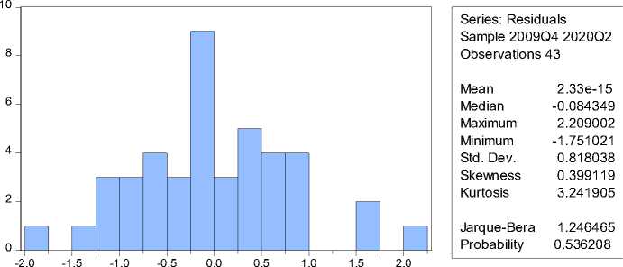
Gambar 4. Uji Normalitas

• 1.    Serial correlation test

To detect correlations between observation members using time series data, it is necessary to conduct a serial correlation test. The Lagrange Multiplier test (LMtest) wasused in the serial correlation test in thisstudy. If the probability is more than the value of the α is 0.05, then H0 is accepted which means that there is no serial correlation.

The serial correlation test using the LM test method presented in table 6 shows an F-statistical probability of 0.9281. This probability value of more than 0.05 concludes that H0 which states there is no serial correlation cannot be rejected. That is, there is no serial correlation in residual ARDL (1, 0, 3, 1, 0, 0, 0).

Tabel 6. LM test

F-statistic Obs*R-squared	0.074760 0.220564	Prob. F(2,29) Prob. Chi-Square(2)	0.9281 0.8956
F-statistic	0.654665	Prob. F(11,31)	0.7684
Obs*R-squared	8.105912	Prob. Chi-Square(11)	0.7038
Scaled explained SS	6.269363	Prob. Chi-Square(11)	0.8548

Source: Research results (appendix 21)

• 1.    Discussion

As a phenomenon of monetary-fiscal combination, inflation volatility is seen from a combination of monetary and fiscal factors, namely the money supply, interest rates, exchange rates, tax revenues, government spending, and foreign debt. Assuming ceteris

paribus,here is an analysis of the results of this study estimate.

First, the money supply coefficient is 0.200892 with a probability of 0.0070 (less than 0.05). This suggests a 1 percent increase in money supply growth would lead to inflation of 0.2 percent and a confidence level of 99.3 percent. In

conclusion, the money supply plays a positive and significant role in explaining inflation in Indonesia. Relatively similar results are also obtained in long-term estimates.

The long-term money supply coefficient is 0.258532 with a probability of 0.0024. This means a 1 percent increase in the money supply would increase 0.26 percent inflation with a confidence rate of 99.76 percent. The money supply in the long term has a positive and significant effect on inflation in Indonesia.

This finding proves the research hypothesis that the money supply plays a role in explaining inflation volatility as a monetary-fiscal combination phenomenon in Indonesia. The amount of money in circulation in a country's economy has a positive impact on national inflation. Increasing the money supply will increase people's purchasing power. If this is not followed by an increase in production, there will be an excess of demand that will trigger producers to raise the price of their products, causing inflation. Thus, the occurrence of inflation volatility in this case is due to demand pull inflation.

In this regard, the growth of the money supply should not be higher than the ability of the producer to increase its aggregate supply. In other words, BI as a central bank and controller of the money supply in Indonesia plays an important role in controlling inflation volatility in the country.

The results of this study are in line with Rizqiansyah (2019), Ginting (2016), Trisdian et al. (2015), Saputra and SBM

(2014),and Maggi and Saraswati (2013) which found that the amount of money circulating had a significant positive effect on theinflasi di Indonesian. Darrat (1985) said the growth of the money supply had a rapid and strong positive impact on inflation in Saudi Arabia. Al-Omar (2007) stated a longterm cointegration link between inflation and the money supply in Kuwait. Azhar et al. (2019) found the money supply (M2) had a significant positive effect on the long term although negative was not significant in the short term.

Second, the interest rate coefficient is 1.671093 with a probability of 0.0014 (less than 0.05). This means that interest rates have a positive and significant effect on inflation in Indonesia. A 1 percent increase in interest rates triggered inflation of 1.67 percent and a confidence rate of 99.86 percent. Different effects can occur due to interest rates in the past 1 and 3 quarters. Interest rates in the past 1 and 3 quarters had coefficients of -1.475898 and -0.970622 with probabilities of 0.0499 and 0.0432 (less than 0.05). That is, interest rates in the last 3 and 9 months just have a negative and significant effect on inflation this month. However, in short-term estimates it was found that the negative effect of interest rates on inflation was not significant.

Current interest rates and the previous 2 quarters in the short term have a positive effect on inflation. This month's interest rate coefficient is 1.671093 with a probability of 0.0001 and the interest rate coefficient 6

months ago was 0.970622 with a probability of 0.0162. This means that in the short term a 1 percent increase in interest rates this month increases 1.67 percent of inflation with a confidence rate of 99.99 percent. The 1 percent increase in interest rates six months ago also played a role in explaining the current 0.97 percent inflation with a confidence rate of 98.38 percent. Relatively similar results are also provided by long-term estimates.

The long-term interest rate coefficient is 0.619949 with a probability of 0.0269. A 1 percent increase in interest rates over the long term would increase 0.62 percent inflation with a confidence rate of 97.31. Interest rates play a positive and significant role in influencing inflation in Indonesia, both in the short and long term.

This finding proves the research hypothesis that interest rates play a role in explaining inflation volatility as a phenomenon of monetary-fiscal combination in Indonesia, although it gives different results than the theory. The policy of raising interest rates theoretically aims to lower the inflation rate. The results of this study show that rising interest rates are not effective in lowering inflation in Indonesia. The impact is quite the opposite. Rising interest rates will increase the cost of production and investment earned through banking credit, thus triggering the produsen to raise the price of its commodities. Thus, the occurrence of inflation in this case is caused by cost push inflation.

The results of this study are in line with Azhar et al. (2019) which suggested that interest rates have a significant positive effect in the short and long term in West Sumatra. Likewise Ginting (2016) found interest rates to have a significant positive effect on inflation in Indonesia, both in the long term.pendek maupun long-term. It is clear that high interest rates are actually driving inflation higher in Indonesia.

Third, the exchange rate coefficient is 0.084216 with a probability of 0.0283 (less than 0.05). It showed a 1 percent increase in the exchange rate would lead to inflation of 0.08 percent and a confidence level of 97.17 percent. That is, the rupiah exchange rate on the U.S. dollar has a significant positive effect on inflation in Indonesia.

Relatively similar results are also found in short-term estimates, but are different from long-term estimates. In the short term, the exchange rate has a significant positive effect on inflation in Indonesia. While in the long run the effect of the exchange rate is still positive but not significant.

This finding proves the research hypothesis that exchange rates play a role in explaining inflation volatility as a phenomenon of monetary-fiscal combination in Indonesia. Changes in the rupiah exchange rate over the U.S. dollar have a positive impact on inflation in Indonesia, although not significant in the long run. The increase in exchange rates will make imported commodities more expensive and export commodities cheaper in international trade. If producers have a

factor of production derived from imported commodities, then the increase in exchange rate will increase the cost of production. This will encourage producers to raise the price of their commodities(cost-push inflation).

The increase in exchange rates makes foreign consumers able to buy export commodities cheaper than usual. This enables increased sales and profitability as well as the competitiveness of local companies in international markets. This is what in the long run will reduce the significance of the positive impact of the exchange rate on inflation in Indonesia.

The positive effect of exchange rates on inflation is in line with the results of research rizqiansyah (2019), Ginting (2016), Utami and Soebagiyo (2013),aswell as Saputra and SBM (2014). They found that the exchange rate had a positive and significant effect on inflation in Indonesia.

Fourth, the tax revenue coefficient is -0.029305 with a probability of 0.0645 (over 0.05). It showed an increase in tax receipts of 1 percent could potentially lower inflation by 0.03 percent with a confidence level of 93.55 percent. That is, tax revenue negatively affects inflation, but not significantly at an error rate of 5 percent. The same conclusion was also obtained in longterm estimates, where tax revenues have a negative but insignificant effect on inflation in Indonesia.

This finding is different from the research hypothesis that tax revenue plays a role in explaining the volatility

of inflation in Indonesia. Increased tax revenues due to the increase in rates will decrease people's purchasing power, because of the reduced income they can spend. This decrease in purchasing power will reduce the income of producers, so they will decrease their production and investment, and may even lower the price of their products. In the end, this will lower inflation.

Ideally, the increase in tax revenues has a significant effect on the decline in inflation. In fact, an increase in tax revenues has the potential to menurunkan inflasi, namun tidak signifikan. Tidak signifikannya pengaruh negatif dari penerimaan Taxes on inflation show that there is still no effective implementation of tax policy in this country. Supposedly, an increase in tax revenues that reflects the policy of increasing the tax rate levied by the government should be able to significantly reduce inflation, and vice versa.

The results of this study are in line with the findings of Azhar et al. (2019) which examined regional inflation in West Sumatra. Its findings concluded that tax revenues negatively negatively affect inflation in the province, both in the short and long term.

Fifth, the government spending coefficient of -0.030423 with a probability of 0.0389 (less than 0.05). It showed a 1 percent increase in government spending would lower 0.03 percent inflation and its confidence level by 96.11 percent. That is, government spending has a significant negative effect on inflation in Indonesia.

The significance of the negative influence of government spending on inflation is diminishing in the long run. Long-term estimates show government spending negatively impacts inflation with a confidence rate of 94.78 percent. That is, the error rate is more than 5 percent.

The findings are in line with the research hypothesis that government spending plays a role in explaining inflation volatility as a monetary-fiscal combination phenomenon in Indonesia, although it differs from the theory. An increase in government spending would theoretically increase inflation due to an increase in the money supply. The results showed that increased government spending did not necessarily lead to inflation, although the money supply increased.

Price increases are not only influenced by the money supply. Production costs play an important role in the determination of commodity prices. Although the money supply increases due to increased government spending, the cost of production does not increase significantly, it will not have a positive impact on the price of the commodity produced.

The negarif influence of government spending on inflation was also found azhar et al. (2019),but differed in terms of its significance. Its findings suggest government spending has a significant negative effect in the long term and negarif is insignificant in the short term.

Sixth, the coefficient of foreign debt is 0.097703 with a probability of 0.0805 (more than 0.05). This means a

• 1    percent increase in foreign debt plays a role in 0.1 percent inflation with a confidence level of 91.95 percent. That is, foreign debt has a positive but insignificant impact on inflation in Indonesia. A slightly different conclusion is drawn from long-term estimates.

The Indonesian government's external debt in the long term has a significant positive effect on inflation in the country. The coefficient is 0.125736 with a probability of 0.0283. This means a 1 percent increase in foreign debt would increase 0.13 percent of inflation in the long run with a confidence level of 97.17 percent.

These findings prove the research hypothesis that foreign debt plays a role in explaining inflation volatility as a combination phenomenon. monetary-fiscal in Indonesia. Government external debt that arises due to budget deficits will push inflation higher in the long run. Budget deficits and foreign debt are mutually affecting (Satrianto, 2015). The more the government budget deficit, the greater the amount of foreign debt and the higher the inflation that occurs in the country.

One way to overcome the increase in foreign debt is to seek tax revenues greater than the expenditure that must be spent by the government. This prompted the government to increase the tax rate. The increase in the tax rate will increase production costs for producers. Furthermore, producers will raise the price of their commodities to cover the increase in production costs. Thus, the positive

effect of foreign debt on inflation in this case is due to cost push inflation.

The results of this study are in line with the findings of Hutauruk et al. (2015) which stated that inflation in Indonesia is explained positively and significantly by its government debt budget. Hervino (2011) also found that in the long run, foreign debt positively affects inflation volatility in Indonesia.

A common conclusion that can be taken is that as a phenomenon of monetary-fiscal combination, there is a significant role of the money supply (positive), interest rate (positive), exchange rate (positive), and government spending (negative) in explaining inflation volatility in Indonesia. Tax revenues and foreign debt also play a role, although not significantly.

In the short term, inflation in Indonesia is significantly and positively affected by interest rates and exchange rates. While in the long run, interest rates, money supply, and foreign debt predominantly have a significant positive effect on inflation in Indonesia. Exchange rates, tax revenues, and government spending also contribute to the formation of inflation in the long run, but not yet significant.

This conclusion confirms that inflation in Indonesia is not only influenced by the monetary side in the form of money supply, interest rates, and the rupiah exchange rate against the U.S. dollar as monetarists view. The fiscal side in the form of tax revenues, government spending, and foreign debt also plays a role in explaining inflation volatility in Indonesia.

This is in accordance with John Maynard Keynes's theory that in a country's economic system, inflation is influenced by two things, namely the level of expenditure spent and tax revenues received by the government of the country concerned. When government spending is greater than its tax revenues, then the emergence of government external debt that will ultimately also affect the inflation of the country in question.

In this regard, inflation control through the management of money supply, interest rates, and exchange rates as monetary policy instruments has not been able to fully affect inflation volatility in Indonesia, but there needs to be a combination with fiscal policy in the form of effectiveness of tax revenues and government spending and minimizing government external debt. Fiscal and monetary policy makers should be able to make appropriate and proportionate policies in controlling inflation in Indonesia.

1. Conclusion

An important point that can be concluded from the results of this study is the money supply, interest rates, exchange rates, and government spending in general play a significant role in explaining inflation volatility as a phenomenon of monetary-fiscal combination in Indonesia. The positive influence of interest rates dominates inflation in the short and long term. In addition to interest rates, the positive influence of the money supply and foreign debt also predominantly affects inflation in the long run. This

means that inflation volatility in Indonesia is dominated by interest rates from the monetary side and foreign debt from the fiscal side. Tax revenues have not played an effective role in lowering inflation in Indonesia. The implication is that Bank Indonesia needs to streamline policies related to managing interest rates while the government needs to review the effectiveness of tax revenues and reduce foreign debt.

In terms of monetary, the effectiveness of policies related to the management of interest rates in regulating the money supply needs to be increased. Meanwhile, from the fiscal side, further efforts are needed in increasing the effectiveness of tax revenues and government spending to minimize government external debt.

This research analysis is limited to inflation from the money market side, does not analyze inflation from the market side of goods, such as output or economic growth and so on. The variables used in modeling are limited to several key variables that represent monetary and fiscal phenomena. Further research is expected to examine inflation with more variables that vary from the side of the money market and the goods market.

Referensi

Al‐Omar, H. (2007) ‘Determinants of inflation in Kuwait’, Journal of Economic and Administrative Sciences, 23(2), pp. 1–13.

Azhar, Z., Satrianto, A. and Nofitasari (2019) ‘Inflasi dari sudut pandang moneter dan fiskal (studi kasus Sumatera Barat)’, Jurnal Kajian

Ekonomi dan Pembangunan, 1(1), pp. 131–144.

Baqaee, D. R. (2019) ‘Asymmetric inflation expectations, downward rigidity of wages, and asymmetric business cycles’, Journal of Monetary Economics. Elsevier B.V., 9(23), pp. 1– 20.

Berge, T. J. (2018) ‘Understanding survey-based inflation expectations’, International Journal of Forecasting. Elsevier B.V., 34(4), pp. 788–801.

Binder, C. C. (2018) ‘Inflation expectations and the price at the pump’, Journal of Macroeconomics, 58, pp. 1– 18.

Carlstrom, C. T. and Fuerst, T. S. (2000) ‘The fiscal theory of the price level’, Economic Review 2000 Q1, pp. 22–32.

Darrat, A. F. (1985) ‘Inflation in Saudi Arabia: An Econometric Investigation’, Journal of Economic Studies, 12(4), pp. 41–51.

Das, A., Lahiri, K. and Zhao, Y. (2019) ‘Inflation expectations in India: Learning from household tendency surveys’, International Journal of Forecasting. Elsevier B.V., 35(3), pp. 980–993..

Feldkircher, M. and Siklos, P. L. (2019) ‘Global inflation dynamics and inflation expectations’, International Review of Economics and Finance, 64, pp. 217–241.

Ginting, A. M. (2016) ‘Analisis faktor-faktor yang mempengaruhi inflasi:

studi kasus di Indonesia periode tahun 2004-2014’, Kajian, 21(1), 21(1), pp. 37–58.

Gujarati, D. (2015) Econometrics by example second edition. LONDON: PALGRAVE.

Hammoudeh, S. and Reboredo, J. C. (2018) ‘Oil price dynamics and marketbased inflation expectations’, Energy Economics. Elsevier B.V., 75, pp. 484– 491.

Hervino, A. D. (2011) ‘Volatilitas inflasi di Indonesia: fiskal atau moneter?’, Finance and Banking Journal, 13(2), pp. 139–149.

Hossain, A. A. (2010) Bank sentral dan kebijakan moneter di Asia Pasifik. Jakarta: Jakarta: Rajawali Pers.

Hutauruk, N. D. H., Kuncoro, H. and Sebayang, K. D. (2015) ‘Dampak kredibilitas kebijakan fiskal pada inflasi di Indonesia’, in Proceedings Book Seminar dan Konferensi Nasional. Jakarta: Fakultas Ekonomi Universitas Negeri Jakarta, pp. 1–17.

Jahan, S. and Papageorgiou, C. (2014) ‘What is monetarism? Its emphasis on money’s importance gained sway in the 1970s’, Finance & Development, 51(1), pp. 38–39.

Jiranyakul, K. and Opiela, T. P. (2010) ‘Inflation and inflation uncertainty in the ASEAN-5 economies’, Journal of Asian Economics, 21(2), pp. 105–112.

Jongwanich, J. and Park, D. (2009) ‘Inflation in developing Asia’, Journal of Asian Economics, 20(5), pp. 507– 518.

Maggi, R. and Saraswati, B. D. (2013) ‘Faktor-faktor yang mempengaruhi inflasi di Indonesia: model demand pull inflation’, Jurnal Ekonomi Kuantitatif Terapan, 6(2), pp. 71–77.

Montes, G. C. and da Cunha Lima, L. L. (2018) ‘Effects of fiscal transparency on inflation and inflation expectations: Empirical evidence from developed and developing countries’, Quarterly Review of Economics and Finance. Board of Trustees of the University of Illinois, 70, pp. 26–37.

Orlowski, L. T. and Soper, C. (2019) ‘Market risk and market-implied inflation expectations’, International Review of Financial Analysis. Elsevier, 66, pp. 1–8.

Rizqiansyah, M. F. (2019) Pengaruh kebijakan fiskal dan moneter terhadap inflasi di ASEAN-3. Universitas Jember.

Rumler, F. and Valderrama, M. T. (2020) ‘Inflation literacy and inflation expectations: Evidence from Austrian household survey data’, Economic Modelling, 87, pp. 8–23.

Saputra, K. and SBM, N. (2014) ‘Analisis faktor-faktor yang mempengaruhi inflasi di Indonesia 2007-2012’, Diponegoro Journal of Economics, 3(1), pp. 1–15.

Satrianto, A. (2015) ‘Analisis Determinan Defisit Anggaran Dan Utang Luar Negeri Di Indonesia’, Jurnal Kajian Ekonomi, 4(7), pp. 1–25.

Soybilgen, B. and Yazgan, E. (2017)

‘An evaluation of inflation expectations in Turkey’, Central Bank Review, 17(1), pp. 31–38.

Surjaningsih, N., Utari, G. A. D. and Trisnanto, B. (2012) ‘Dampak kebijakan fiskal terhadap output dan inflasi’, Buletin Ekonomi Moneter dan Perbankan, 14(4), pp. 389–420.

Trisdian, P. A., Pratomo, Y. and Saraswati, B. D. (2015) ‘Volatilitas inflasi daerah di Indonesia: fenomena moneter atau fiskal?’, Jurnal Studi

Pembangunan Interdisiplin, 24(1), pp. 76–89.

Tutino, A. and Zarazaga, C. E. J. M. (2014) ‘Inflation is not always and everywhere a monetary phenomenon’, Economic Letter, 9(6), pp. 1–4.

Utami, A. and Soebagiyo, D. (2013) ‘Penentu inflasi di Indonesia; jumlah uang beredar, nilai tukar, ataukah cadangan devisa?’, Jurnal Ekonomi & Studi Pembangunan, 14(2), pp. 144– 152.

324