Trafic Signs Detection Based On Saliency Map Using Canny Edge

Journal of Electrical, Electronics and Informatics, Vol. 2 No. 1, February 2018

1

Trafic Signs Detection Based On Saliency Map Using Canny Edge

Putri Alit Widyastuti Santiary¹, I Made Oka Widyantara², Rukmi Sari Hartati³

• ^1,2,3Master of Information Systems and Computer, Electrical Engineering Graduate Program Udayana University

Denpasar, Bali, Indonesia

¹[email protected]

²[email protected]

³[email protected]

Abstract This paper proposed Canny edge detection to detected saliency map on traffic sign. The edge detection functions by identifying the bounds from an object on an image. The edge of an image is an area that has a strong intensity of light.The pixel intensity of an image changes from low to high values or otherwise. Detecting the edge of an image significantly will decrease the amount of data and filters insignificant information by not deleting necessary structure from the image. The image used for this paper is a digital capture of a traffic sign with a background. The result of this study shows that Canny edge detection creates saliency map from the traffic sign and separates the road sign from the background. The image result tested by calculating the saliency distance between a tested image and trained image using normalized Euclidean distance. The value of normalized Euclidean distance is set between 0 to 2. The testing process is done by calculating the nearest distance between the tested vector features and trained vector features. From the examination as a whole, it can be concluded that road sign detection using saliency map model can be built by Canny edge detection. From the whole system examination, it resulted a accuracy value of 0,65. This value shows that the data was correctly classified by 65%. The precision value has an outcome of 0,64, shows that the exact result of the classification is 64%. The recall value has an outcome of 0,94. This value shows that the success rate of recognizing a data from the whole data is 94%.

Index Terms— traffic signs, saliency map, Canny edge detection, normalized Euclidean distance.

II. INTRODUCTION

The automatic traffic signs detection is an interesting topic on intelligent transportation systems and has been implemented on various applications such as driving safety and automatic vehicle guidance. Traffic signs can be in the form of symbols, letters, numbers, sentences or combinations and serves as warning, prohibition, command or directions for road users [9]. The problem of traffic sign recognition has some beneficial characteristics such as unique design of traffic sign board, which means the sign shape variations are small, and significantly color contrast against the environment [18].

Traffic sign detection by real time and accurate has become an attention in Computer vision practices. Computer vision aims to computerized human vision or create digital images from original images (based on human vision). The aim of traffic lights detection system is to guide and give directions to drivers while driving, thus increasing the road safeness. This system can be classified into two parts, which are a system that provides information to

drivers and system that acts all at once for the vehicle. [8].

Traffic signs are designed to be salient from the objects around them or background. The computation methods to automatically detects those traffic signs in the image remains significant. Humans can identify salient areas in their visual fields with surprising speed and accuracy before performing actual recognition. Computationally detecting such salient image regions remains a significant goal, as it allows preferential allocation of computational resources in subsequent image analysis and synthesis [3]. The objective is to separates the desired objects from the background around the image. This study proposed Canny edge detection to obtains saliency map model of traffic signs detection.

• II . CANNY EDGE DETECTION

The objective of edge detection is to identify the boundaries of an object inside image. The edges of an object are areas that has a strong light intensity. The pixel intensity of an object changes from low to high value or vice versa.

Detecting the edges of an object significantly reduce the amount of data and filter out useless information without loss important of structure of the image. One of the modern edge detection algorithms is edge detection using the Canny method.

Canny edge detection detects the actual edges with minimum error rate. Canny operators are designed to produce optimal edge image output. The Canny edge detection algorithm as follows [15]:

1. Application of Gaussian filter to reduce noise.

This process produces an image that looks a bit blurry. It aims to get the edge of the real object. If not applied, the fine lines will also be detected as edges. Here is one example of a Gaussian filter with σ = 1.4 below.

	2	4	5	4	2
	4	9	12	9	4
—	5	12	15	12	5
115	4	9	12	9	4
	L2	4	5	4	2-∣

2. Edges value detection.

Finds the edge value by connecting the image gradient using a pair of 3x3 convolution matrices Gx and Gy below. Gx predicts the gradient value for x direction (column) and the other predicts the gradient value for the y direction (row).

I

1

2

1

0+1

0+2

0+1

Gx

+1+2

I00

L -1-2

Gy

+1 0 +1

I

The edge gradient G calculated by equation (1):

G — G_x + Gy

(1)

3. Edges direction detection.

Finds the edge direction θ using equation (2):

In above matric, (a) pixel has four possible directions when looks into surrounding pixels. The directions are as follow: 0^o horizontal direction, 45^o positive diagonal direction, 90^o vertical direction, and 135^o negative diagonal direction. Hence, the edge should point into the four directions, depends on which direction is closest. For example, if the angle is 3^o, its became 0^o. The next step, divide into four colors so that the lines with different directions will have different colors. The divisions as follow: (0^o - 22.5^o) and (157,5^o - 180^o) is yellow, (22.5^o -67.5^o) is green, and (67,5^o - 157,5^o) is red.

• 5.    Non-maximum suppression process.

Non-maximum suppression is used to trace edge within edge direction and filter out pixels unconsidered as edge. This will show a fine line on the output image.

• 6.    Binary with applying two thresholds.

• III.    RESEARCH METHODE

The dataset used in this study are digital images of traffic signs from image dataset at URL http://aganemon.tsc.uah.es/Investigacion/ gram/traffic_signs.html [1]. Dataset contains of 325 images and processed using Java programming language. Computer program runs on portable computer with dual-core T2080 processor 1.73 GHz 1GB memory. In Figure 1 below shows process flow diagram.

• A. Input Image

The input- image has some characteristics that came from shooting conditions. Distance shooting made differences of close or long-distance nput-image. Lighting condition made input-image bright or dark. Shooting orientation showed that images are shoot at different orientations. Not all images at perpendicular position, there are some images shoot at a somewhat skewed position.

θ — arc tan (∣^)

(2)

4. Edges direction connection.

The directions of the edges are connected in a direction that can be traced according to the original image. The following example uses a 5x5 pixel image.

(2.11)

x	x	x	x	x
x	x	x	x	x
x	x	a	x	x
x	x	x	x	x
x	x	x	x	x

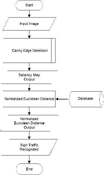
Figure 1. Proces Flow Diagram

• B.    Canny Edge Detection

Edge detection of traffic signs used Canny procedure. The edge of an object within image is an area that has a strong light intensity. Intensity of pixel changes from low to high value or vice versa. First, the original image in the r-g-b color space is converted into a grayscale image I with equation (3) [16].

I = (r+ g + b)/3(3)

Second, the grayscale image is filtered by applying a Gaussian filter with σ = 1.4 as follows:

■ 2   4    5     42'

1   4  9  12   94

^{5  12  15  125}

¹¹⁵ 4  9   12   94

-2   4    5    42-

And then, the edge value is obtained by applying two matrices Gx and Gy as below:

Γ-1  0+1

1-2  0+2

-1 0+1

Gx

I

+1 0

-1

+2 +1

00

-2 +1

Gy

• C.    Threshold

Binary image is obtained by applying a threshold. Binary process aims to adjusts intensity of gray level image. It changes image initially a 255-gray level (8 bit) into binary (black and white). Within threshold results become clear.

One thing to consider in threshold process is to chooses a threshold value. Pixels value below threshold value will be set as black otherwise as white. The threshold value T is calculated by using equation (4) [15].

ψ _ f maks⁺ f min

2

(4)

Images result of binary process is final result of saliency map.

• D.    Normalized Euclidean distance

Normalized Euclidean distance from cropped test-image results of saliency map compared with train-image dataset. The normalized Euclidean distance of two vector feature of u and v is shown by equation (5) [13].

d(u,v) = (∑i(u_i - v_i)²)^v2

(5) with,

“i         v

ⁱ     Hull ^{, i}     HvH

(6)

HvH = [∑iV_i²]^v2

(7) where:

d(u, v) = Normalized Euclidean distance u, v = vector feature.

The smaller of score d(u, v), the more similar of two feature vectors or vice versa. Characteristic of normalized Euclidean distance is that the result within range of 0.0 ≤ d(u, v) ≤ 2.0.

Output image of saliency map is tested by calculates the saliency distance between test-image and train-image in the database. The test results are classified into two types, namely signs and not-signs.

• IV.    RESULTS AND DISCUSSION

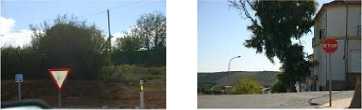
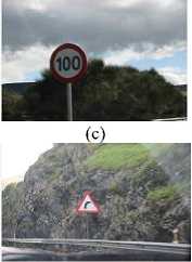
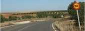
The saliency map in this study has been tested from collection of digital images on dataset. The original image can be seen in Figure 2 (a) through (h) in which have differences type of test data.

(b)

(f)

(h)

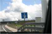
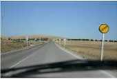
Figure 2. The original images (a) Data 1, (b) Data 2, (c) Data 3, (d) Data 4, (e)

Data 5, (f) Data 6, (g) Data 7, (h) Data 8

Figure remark: Data 1 and 2 are priority signs, data 3 and 4 are prohibition signs, data 5 is a danger sign, data 6 is warning and information sign, data 7 is end of prohibition sign and data 8 is obligation sign.

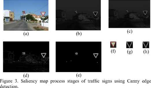
Process stages of obtaining a saliency map for traffic signs using Canny edge detection for data 1 is shown by figure (3).

• 1)    The Original  Images:  Traffic signs image with

background in r-g-b color space. This is used as input data on the system. The original image is shown in Figure 3 (a).

• 2)  Grayscale: Converts the r-g-b original images into one

grayscale image. Each intensity values of color channel are summed up into a grayscale image I. And then obtains the absolute averaged value of I by eliminates decimal values. Grayscale conversion produces a new different gray level image. The image has various level of black to white. Grayscale conversion results are shown in Figure 3 (b).

• 3)    Gaussian filter: Applied a Gaussian filter to noise reduction. The grayscale image filtered with a Gaussian filter with σ = 1.4. This process produces a bit blurry image. The Gaussian filter results are shown in Figure 3 (c).

• 4)    Canny Edge Detection: Canny edge detection finds the edge value by connecting image gradient using a 3x3 convolution matrix pair. The result of Canny edge detection is shown in Figure 3 (d).

• 5)    Binaryization: Binary images obtained by applying two thresholds. This is final stage to gets the saliency map of traffic signs image. The result of the binary process is shown in Fig. 3 (e).

• 6)  Cropping: Cropping process for original image and

saliency map image result. Cropping separates image object from its background. Cropped results used to calculate the normalized Euclidean distance between the test-data and the train-data. Figures 3 (f), 3 (g), and 3 (h). show cropped original image, test-data and comparison data. Cropped test-data results of the saliency map process. Comparative data are train-data, in which results of a saliency map processes that has been stored in database.

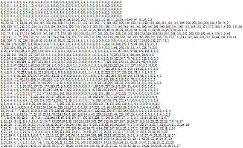
• 7)    Normalized Euclidean Distance: For assessment of result normalized Euclidean distance of cropped saliency map image results (test-data matrix) compared with training data (train-data matrix) using equation (5). Test-data matrix of Data 1 can be seen in figure 4 and figure 5 for train-data matrix.

::::-::.-..--..■■.........■............j

A₁A₁A₁A₁A₁X XA₁O₁J₁I₁1, l,∣_tl_tA₁ -J₁O₁O₁J₁ Ri₁⁴J₁XA₁O₁O₁O₁A_lA₁O₁C₁C₁A₁A₁O₁O₁J

A A A A A A A A C-. C₁X A A C C₁1₁XA⁴₁⁴ .A I, C, C₁C₁A A C. C₁C₁A A C C₁C₁A A C-. C₁J

Xl K^a₁UMCf₁S⁴₁Sl₁^aJ₁K₁CI..

ihm,;

2W.JJI,XSAX.t^aJ₁ NA IAi UX IJl₁Ill ICa lit U

KiKi!

• • ICZ ZW ICX M₁HS_tWI₁Zi. S. J₁ >, 4.t.C A > C. C. !.J₁A₁J₁I₁I₁X XC CA ! « NMJJ.tJ.UJ, ZV⁴I₁C i s i v »i, iχ ∣^af ,3χ icmjv M₁AA⁴₁ «,a xmc-aaj,ua IU_lUjs^a_lHj v iq,h«j«:Au

* 1 SJ_lUi_l κ₁w_tιr_ta'jχ uc.c.Ajj_tc_tc_tu Ae,o,θAxι_to_tθA ⅞ i∙^aχw∣_t∣^afXR∣so₁3WM₁A⅛_tc XM-MK UC JMU₁HS ISC U_tC₁J₁J J₁C₁J₁AM JCJJ M₁M X “ AJ N^a X,t Mi₁IlJ₁J₁X JC H n J₁ K₁ IH. IH. U₁IS^a₁HlHJ_tCA₁J₁J₁J₁JA MJ_tCA₁J₁CJJ₁I, 'Ill₁ISM⁴MMSC₁XtVAXC XXXlJ^a IH IllAi₁HiIJ^a K 1 J. X₁X₁J₁Ia M J CJ₁J₁J₁I₁C₁J K IlXUl₁M₁ Ill₁H^a IN Xl₁IC₁C 4 XAA W. Γ4.2ll, SJ₁Ul I5S,U1AC₁CA, SJ.C. JA₁AC-JJJ AC.^a. IX 235, ISI,«Alt ISAJJ₁JJ_tS₁AO 1 A X X X VJlJ₁UA IS, Hi UI₁SjJAIC₁C₁X XC C C 1. IJJJ₁SJ Ui, JI^a₁I^a₁ IZ₁Jil TjA I₁X₁A X

J J J₁J₁J₁1 t^a₁t^4a. ZU₁ ^aJ IX₁I¹M^aIIJ₁C₁C₁J J C C.l t, JJJ₁ UlX₁HMW_tV₁ ItC₁ISMS₁ IC₁C₁A J₁ C.C X i AAUtl_tSC Si U- Ji I^aA₁HXrt₁XC₁C₁X JCiiJ Xf₁UIZ Il^a₁⅛ UlUAU ⁴ J J XC₁C₁X S A A J₁ J₁A J₁ JJ₁M₁ HS₁IZI₁JIA⁴S JW₁⁴S₁I₁C₁J J C. C. C A J₁IA t JA IS! IW^4a_lZIt. I5β₁ll₁l, JJ₁C_tCAtC ..                    -  ,          .∙   ...₁₁₁         ,

SJA₁XAJJ₁ J₁J₁^aMa_iIM IC₁Ir_iISJ₁K₁I₁A S₁C₁1₁J t₁ N₁IKlK₁^aI₁^aI_tIS⁴₁UR II_tIJ₁C₁C₁M₁ J₁I₁I t a AAAAAA⁴₁IMX₁UA ICl^aMSM^aMJ JJCi M₁^aSHJlF IM^aXHH^aJ C J J Ji₁C₁X 1 ⁴ 1¹- ⁴J₁⁴, UA₁A_tC-C₁S₁ W₁ZCAlJt_t I^aS₁IS¹ .t∏ 11.C₁C₁0₁ASO_tIMIS! ^aA IJl₁NS₁IZC₁⁴ AA⁴_tI₁A, S₁ SJ₁J₁I II₁Mj₁IA C-A XXf₁SMN₁IJX-HXUl₁F J J A», I l^a₁ ISJ₁Ut₁ H IM₁JM₁N₁X X X C i a a A UM

^{a a} M, 1 IC. HSJA₁ ^a₁ U₁IS₁NS₁S⁴₁ WA⁴S IM F. IX l-'MH.M. I* NM^a 1' U₁I. JJ₁ H, XU₁U₁U. IlMA₁Ilj₁U ∣A^a Al H^a₁XiiS UMXI₁UMCX^a IlMMJ^a₁U^a S₁U J' 1 i I W₁JSLtJ₁ I^a₁IS₁W₁IJ₁IAH UkS_tX₁JX HC₁XJ₁ IJS.IMTA15Iie.il, IAIC_tZJS 'S,U,11,11 ^a N₁Jl₁ IC-, lS_ς l^a JJ₁H₁IIS₁J₁IS, Jl J^a₁ F,l⅛ JSC- XC JX W, Ii A M Uj IS^a₁H₁S₁ U₁S It₁Jl₁JX

S₁ 3,JlS₁ M,∣l.U.^a.S.ZMJ IJ₁W₁ISMSt.J⁴C-I₁^aMWAr ^aA X.tS.ll.lJ. 1" Sl₁S₁II₁ JJ₁MMJ I.’ I₁JJ

I J^a₁JMAXU I Xi S ^{a a} IJ₁Ii U₁U^a₁NJM 11H IMUi ISC H U IC₁JlU U₁U K l>,J^a M₁H₁JC UIS₁J^a

1 F₁JSJJ₁J₁ S₁I₁J₁J₁ 5. Z ^a.lS. II₁II F.SS UJ-UiIJt₁I-⁴I₁HZ M IJ₁J₁U₁W_tS₁C₁S₁IZlAC₁SI₁IMMAJ^a₁U .■•-■.                               . . u» .u ιcx∣∙ :« :. :; i t: H ., ,. .- -    .

Figure 4. Test-data matrix.

TABLE 1

Normalized Euclidean Distance Result

No	Data	Euclidean distance	Recognized as
1	Data 1	0,0819	Sign
2	Data 2	0,0326	Sign
3	Data 3	0,0424	Sign
4	Data 4	0,0913	Sign
5	Data 5	0,0377	Sign
6	Data 6	0,1880	Sign
7	Data 7	0,1451	Sign
8	Data 8	0,3848	Sign

rcxΛ λCΛ.r>Λ< J» :«.:r a.uuι^j

H.C.J J 4,4 C X J ιi IIkIM IC-4' ^I ₁ Q₁UA₁S₁C_tC₁CAAJ₁IS₁JSJ₁ Iflft II₁UlIS ,K₁J₁IXCJ₁J₁I₁ M₁ICiJK₁IALlW₁ISk .t’»,t»,sa₁c₁j.i>•’* 2’ ιr.w.fiπι∣ 5i_llll, n 4 ,C C S, X₁IM lit, 'S IJl₁MX IS

r_lιιa₁a₁u₁A₁∞₁iH,¾ w.bs.hm». ∞ji 4₁s,τ,i4 Ia₁Mkcskc₁Mkiw r ικ_l3iut,>2 t.π.s.L^, n • c ir.xs t’, tjsjs∙.υ>:« :r i ^_tU,>S Ii U₁M₁X₁IMU₁M₁IM, Il It XU Jlt □ ,∏.1 ld,J.IJ₁KI', ST₁HllSt.M₁JIM’S, S₁MJ Ii,-, x n ji i.«,«,Ui_lIM₁IM j > IM S- u: I iJj.-. -::.::.u. ir.»st,u. Siw ihj« ; J₁XXl is u i!.Si_lXuujiajiiKiU iK; jsa.-a -, U.K.».::, 11, MJ.isi s»», ir.ucm i UJX₁>ι₁M,a,J>₁z z.u,xjj,Mji4jM m,m

5, J₁ U. IM₁IMAl₁ IS₁MS₁IK₁Il₁CA SA₁C₁JA X4 J,t A 3 1.«.«A. S CAX WIK TM₁Ml1».JJJ₁O λ λ λ < IU₁ IM_lU_aU?.XiM 1 C₁X i X JJA X IJ 4 X X 4 4 4.1 * U1,X5. UX IS_k IK₁XCk -I- XC₁C

5, Λfl⅛ If₁UI₁III₁ M,ai IF₁M₁ IAA», J₁JA LI₁J₁OA XJ₁ LC₁A M₁JIS₁JII₁M₁ lll.a'. IX₁A 1,AC₁C ∖X,XX K₁IU₁Ill₁ S UllM UikC₁C₁XSJ₁CJJ₁ XCJ JjXC 'JXXS_kUl M₁XIl₁ IiXJi JJ₁X XC

SAflA ITO_tIU_tIMIS_kSlin,9β,I S J,C.C.S₁ S₁C₁O₁O₁I, I 4.4. J₁SlISl II’,J’, 150.31, ’J A * l,*.S.i

J J • » JICJU,XJM ICOJM₁IttJl X₁C₁Cj XC₁CJj₁LC_tC C₁XlJS_iXS₁Al SC XlS I-XlSJJ₁J 1 4„

S, S₁Afll t,z<.tsi Ml IAIIfl₁MllILT_tAS₁CAA₁A 14.1 J t, 1»4 Hllflt A MiLlJO₁T₁Zi AC₁C₁L t

J₁ J₁ J₁ X X⅛∏₁u∙, Xi₁-X₁ IM₁XS l∙i⅛C,CΛ X4.C I: X ’ « A iκ,M5, IX₁MJlC WJ m IC₁CA XC₁I

t j.tt.tt. 1». u,», zo.r. u, n it. ? is, i IM₁ICk Ill₁IlS₁ Iil Iil US ISC₁I-J IM IS Itt₁XIXIX₁Ill ZlkJU₁XMl Wl₁ Iflt I SJX₁-C₁JI) JLS₁Il₁JXa M 4X44 44 ' ∙.!∙t ∏5.1∏, U1.3M.ΣUIFAC 144.1. MXlM₁HXJiJ jl⅛JX 111 Itk IM₁IL

Figure 5. Train-data matrix.

Table 1 shows results of normalized Euclidean distance of all data. The normalized Euclidean distance values in range of 0.0 and 2.0. It shows both data have slight different, but still recognized as a sign. From the whole system examination, it resulted a accuracy value of 0,65. This value shows that the data was correctly classified by 65%. The precision value has an outcome of 0,64, shows that the exact result of the classification is 64%. The recall value has an outcome of 0,94. This value shows that the success rate of recognizing a data from the whole data is 94%.

• V.    CONCLUSSION

This study has demonstrated that the application of Canny edge detection performs clear of edge detection results. The saliency map model of traffic signs detection has well generated with Canny edge detection and produce great sign identification. From the whole system examination, it resulted a accuracy value of 0,65. This value shows that the data was correctly classified by 65%. The precision value has an outcome of 0,64, shows that the exact result of the classification is 64%. The recall value has an outcome of

0,94. This value shows that the success rate of recognizing a data from the whole data is 94%.

REFERENCES

• [1]    Bascón, Saturnino Maldonado. 2007. Road-Sign Detection and Recognition Based on Support Vector Machines. IEEE Transactions On Intelligent Transportation Systems, Vol. 8, No. 2, June 2007.

• [2]    Borji, Ali dan Laurent Itti. 2013. State-of-the-Art in Visual Attention Modeling. IEEE Transactions On Pattern Analysis And Machine Intelligence, Vol. 35, No. 1, January 2013.

• [3]    Gao, Shangbing dan Yunyang Yan. 2012. Salieny and Active Contour based Traffic Sign Detection. ISSN 1746-7659, England, UK Journal of Information and Computing Science Vol. 7, No. 3, 2012, pp. 235240.

• [4]    Hechri, Ahmed dan Abdellatif Mtibaa. 2011. Lanes and Road Signs Recognition for Driver Assistance System. IJCSI International Journal of Computer Science Issues, Vol. 8, Issue 6, No 1, November 2011.

• [5]    Itti, L., Koch, C. dan Niebur, E. 1998. A Model Of Saliency-based Visual Attention For Rapid Scene Analysis. IEEE Transactions On Pattern Analysis And Machine Intelligence Volume 20, Issue 11, Nov 1998.

• [6]    Itti, L. 2004. Automatic Visual Salience. Scholarpedia, 2(9):3327, 2007.

• [7]    Jayachandra, Chinni. dan H.Venkateswara Reddy. 2013. Iris Recognition based on Pupil using Canny edge detection and K-Means Algorithm. International Journal Of Engineering And Computer Science ISSN:2319-7242 Volume 2 Issue 1 Jan Page No. 221-225.

• [8]  loy, gareth. 2004. fast shape-based road sign detection for a driver

Assistance System. Computer Vision andActive Perception Laboratory Royal Institute of Technology (KTH).

• [9]    Menteri Perhubungan RI. 2004. Rambu Lalu Lintas.

• [10]    Neibur, Ernst. 2007. Saliency Map.

• [11]    Parikh,N, L Itti, dan J. Weiland. 2010. Saliency-Based Image Processing ForRetinal Prostheses . Journal Of Neural Engineering J. Neural Eng. 7 (2010) 016006 (10pp).

• [12]    Polatsek , Bc. Patrik. 2015. Spatiotemporal Saliency Model Of Human Attention In Video Sequences (Thesis).

• [13]    Powers, David M W. 2011. Evaluation: From Precision, Recall and F-Factor to ROC, Informedness, Markedness & Correlation. Journal of Machine Learning Technologies (2011) 2 (1): 37-63 [online].

• [14]    Putra, Dharma. 2010. Pengolahan Citra Digital. Yogyakarta: Andi.

• [15]    Putra, Dharma. 2009. Sistem Biometrika. Yogyakarta: Andi.

• [16]    Rambe, SJ. 2011. Bab 2 Landasan Teori Citra Digital.

• [17]    Treisman, Anne M. dan Garry Gelade. 1980. A Feature-Integration Theory Of Attention. Cognitive Psychology, vol. 12, pp. 97-136, 1980.

• [18]    Won,Woong-Jae, Sungmoon Jeong, dan Minho Lee. 2007. Road Traffic Sign Saliency Map Model. Proceedings of Image and Vision Computing New Zealand 2007, pp. 91–96, Hamilton, New Zealand.

• [19]    Zhang, Jianming dan Stan Sclaroff . 2013. Saliency Detection: A Boolean Map Approach. Journal IEEE International Conference on Computer Vision (ICCV).