SHORELINE CHANGE ANALYSIS USING DIGITAL SHORELINE ANALYSIS SYSTEM METHOD IN SOUTHEAST BALI ISLAND
on
Shoreline Change Analysis Using Digital Shoreline… [Fajar Lukman Hakim, dkk]
SHORELINE CHANGE ANALYSIS USING DIGITAL SHORELINE ANALYSIS SYSTEM METHOD IN SOUTHEAST BALI ISLAND
Fajar Lukman Hakim1), Takahiro Osawa2,3), I Wayan Sandi Adnyana4)
-
1) Masters Program in Environmental Science, Udayana University
-
2)Center for Remote Sensing and Ocean Sciences (CReSOS) Udayana University
-
3)Center for Research and Application of Satellite Remote Sensing (YUCARS) Yamaguchi University, Japan
4)Faculty of Agriculture, Udayana University
*Email: fajjar_hakim@gmail.com
ABSTRACT
Based on data from the Bali Public Works Office, in 1987 the abrasion reached 51.50 km, in 2003 it reached 86.5 km, and in 2006 it increased to 140 km. Coastline change research is needed for coastal environmental protection, mitigation, and sustainable development. The objectives of this research are: 1) To predict wind speed and direction for the last 30 years; 2) To measure changes in coastlines over the last 30 years (1989-2020); and 3) Comparison of changes in coastline in 4 periods 1989-2000; 2000-2010; 2010-2020 and 2016-2020. Digital Shoreline Analysis System (DSAS) is a method that works on ArcGIS software which is used to calculate shoreline changes based on time statistics and a geospatial basis. The results of the average EPR in 19892000 (Landsat imagery), the average abrasion value was -10.43 m/y and the average accretion value was 2.35 m/y; 2000-2010 the average value of EPR abrasion was -2.61 m/y and the average accretion value of 2.65 m/y; in 2010-2020 the average EPR abrasion value was -2.72 m/y and the average accretion value was 1.60 m/y while in 2016-2020 (Sentinel Image) the average abrasion value was -4.32 m/ y and the average value of its accretion is 4.50 m/y. The conclusion of this study 1) The average wind speed ranges from 0.2 to 6.4 m/s. Wind direction shows the dominance of the Australian continent (southeast). This shows that the east monsoon is more dominant than the west monsoon; 2) In the last 30 years (1989-2020) shoreline changes can be seen from the EPR graph with an average abrasion rate of -6.39 m/ y and an accretion rate of 3.15 m/y; and 3) Identification results from 1989-2000 the villages of Padangbai and Ketewel experienced extreme accretion and high abrasion; 2000-2010 Padangbai and Jumpai villages experienced high accretion and abrasion; In 2010-2020, Jumpai and Gunaksa Villages experienced high abrasion and moderate accretion, while 2016-2020 experienced high abrasion and accretion in Tangkas and Gunaksa Villages. For further research, it can include additional variables such as tide and wave data to get better results.
Keywords: DSAS, NSM, EPR, Shoreline Changes, Abrasion, Accretion
is affected by tides. The shoreline consists of the lowest receding coastline, the highest tide, and the mean sea level (Cui and Li, 2011). The shoreline changes continuously; changes occur due to the
land's erosion (abrasion) and the addition of land (accretion). The abrasion and accretion process is caused by sediment transport, tides, waves, currents, anthropogenic, and land use(Arief et al., 2011). Based on the Bali Public Works Office, in 2006 the length of the beach reached 427 km, in 1987 the abrasion reached 51.50 km, in 2003 the abrasion was 86.5 km, and in 2006 it rose to 140 km. The Padanggalak Beach area in Kesiman Village, East Denpasar Regency, Denpasar City, is also still experiencing abrasion. Monitoring of shoreline changes is needed for the study of coastal dynamics, protection of the coastal environment, mitigation map, sea transportation and sustainable development of coastal areas (Kasim, 2012; Putra et al., 2015).
The Digital Shoreline Analysis System (DSAS) is a software add-in to Esri ArcGIS desktop 10.4-10.6 that enables a user to calculate rate-of-change statistics from multiple historical shoreline positions. It provides an automated method for establishing measurement locations, performs rate calculations, provides the statistical data necessary to assess the robustness of the rates, and includes a beta model of shoreline forecasting with the option to generate 10 and/or 20-year shoreline horizons and uncertainty bands (USGS, 2021).
The DSAS method has advantages over other analysis methods, including it can be used for a massive area with a large number of transects, can compare changes in coastlines from different years, and can be used to predict changes in the future coastline (Sugiarta, 2018). Nugraha et al., (2017), The results of the analysis of shoreline changes from 1995 to 2015 in
the southeastern island of Bali (Klungkung and Gianyar) are the dominant shoreline changes occurring on the coast of Gianyar Regency. The technology used in this research is remote sensing. This technology can monitor shorelines for several years and be analyzed using DSAS (Digital Shoreline Analysis System) software developed by the USGS (United States Geological Survey). This technology uses Landsat satellite imagery with an accuracy of 30 square meters using the band ratio method. Landsat satellite imagery was used for 30 years, from 1989-2020. The aims of this research will be formulated as to predict wind speed and direction for the last 30 years; measure shoreline changes over the last 30 years (1989-2020), and compare changes in the coastline in 4 periods 19892000; 2000-2010; 2010-2020 and 20162020.
Research locations in the coastal sub-districts of Denpasar City, Gianyar, Klungkung, and Karangasem District. In this study, primary and secondary data were used. Primary data were measured as the present coastline as existing conditions in the research area. Secondary data was interpreted satellite images and wind data by agencies. Data processing was conducted in the last thirty (30) years from 1989-2020. The year of data processing was carried out in 1989; 2000, 2010, and 2020. The dynamical shoreline changes in 1989-2000, 2000-2010, and 2010-2020 are compared to determine the changes.
Table 1. Image Material
|
Citra Satellite |
Acquisition Date (mmm/ dd/ yy) |
Sensor Type |
Resolution (m) |
Path |
Row |
|
Landsat 4 |
Mar/30/89 |
TM |
30 |
116 |
66 |
|
Landsat 7 |
Aug/19/00 |
ETM+ |
15, 30 |
116 |
66 |
|
Landsat 7 |
Nov/19/10 |
ETM+ |
15, 30 |
116 |
66 |
|
Landsat 8 |
May/30/20 |
OLI |
15, 30 |
116 |
66 |
|
Sentinel 2A |
Mar/10/16 |
MSI |
10 |
116 |
66 |
|
Sentinel 2B |
May/12/20 |
MSI |
10 |
116 |
66 |
The Satellite data were processed in the last thirty (30) years from 1989-2020 with the specific acquisition date in Table 1. The year of data processing in 1989, 2000; 2010; and 2020. The results of the dynamical shoreline changes in 19892000, 2000-2010, and 2010-2020 were compared to determine the changes. The Landsat imagery in each year undergoes data processing with the following stages. The first stage of image cutting (cropping Image) to ease the work process of the computer.
The second stage of geometric correction is to improve objects' position in the Image according to the actual situation. The geometric correction with ENVI 5.3 software help regarding the ground checkpoint from the field survey results and Bali's Province's RBI Map. The third stage of radiometric correction is to correct the Image caused by satellite damage (Istiqomah et al., 2016). Radiometric correction using ENVI 5.3 software to sharpen images, while atmospheric correction to eliminate atmospheric disturbances. The fourth stage is the delineation process to separate land and waters in the form of a coastline, which will be analyzed using a composite band technique to display the observed object's boundary (Kasim, et al., 2015).
To change the MNDWI raster data to vector data using the threshold method.
Furthermore, it is digitized by the onscreen digitizing method. The delineation formula with MNDWI for ETM + and TM sensors, according to Xu (2006), is as follows:
MNDWI =
Green-MlR
Green+MIR
……………… (1)
The MNDWI formula for OLI sensors,
according to Luyan Ji (2015), as follows:
MNDWI =
Green-SWlR 1
Green+SWIR 1
………………(2)
According to McFeeters (1996), the NDWI method cannot efficiently reduce signal interference originating from land cover features in built-up areas. Xu (2006) noted that water bodies have a stronger absorption in the SWIR band than in the NIR band and that the built-in class has more significant radiation in the SWIR band than in the NIR band. Based on these findings, MNDWI is proposed, which is defined as:
MNDWI =
p Green-p SWIR p Green+p SWIR
………………(3)
Where SWIR is a reflection of TOA
from the SWIR band. In general, compared to NDWI, water bodies have a more excellent positive value in MNDWI, as water bodies generally absorb more SWIR light than NIR light; soil, vegetation, and built-up classes have
smaller negative values because they reflect more SWIR light than green light (Sun et al., 2012). Xu (2006), For Sentinel-2, the green band has a spatial resolution of 10 m, while the SWIR band (Band 11) has a spatial resolution of 20 m. Thus, MNDWI needs to be calculated at a spatial resolution of 10 m or 20 m. Furthermore, MNDWI 20 m is calculated
as:
MNDWI20m =
P
P
20™-p 11
20™+p 11
(4)
Where 11 is the TOA reflection of Band 11 (SWIR) of Sentinel-2 andP2T is the TOA reflection of Band 3, which is enhanced from Sentinel-2 with a spatial 2∩τπ resolution of 20 m. The value of p is
calculated as the average value of the corresponding 2 x 2 P3 values. Conversely, if the spatial resolution of Band 11 is increased from 20 m to 10 m, then MNDWI becomes 10 m spatial resolution, MNDWI 10 m so that it can be calculated
as:
MNDWI10m =
P3~P
ιom 11
P3+P
ιom 11
(5)
where P 11 The TOA reflectance of Band 11 at 10m is produced by downscaling the original 20-m of Band 11. This is achieved by using the PCA pansharpening method. PCA Pan-Sharpening is an approach based on the component substitution for the original data's spectral transformation (Shah et al., 2008).
DSAS analysis methods used are Net Shoreline Movement (NSM), End Point Rate (EPR), Linear Regression Rate (LRR). NSM is used to calculate the distance of shoreline changes. EPR is used to calculate shoreline change rate (Sutikno, 2014). LRR is used for predicting changes
in the coastline. The prediction is only made in areas that have not yet experienced breakwater development, seawall etc,. The coastline prediction also considers the LRR analysis results if the determination coefficient(R2) has a high value, namely R2> 0.7. The next step is to determine the most appropriate regression model by conducting a regression using the variable X as a year and the Y variable as the distance of shoreline change each year with the baseline. The shoreline changes with DSAS show a positive value (+) when experiencing accretion and a negative value (-) if experiencing abrasion.
WRPlot View is a windrose program for meteorological data. Windrose describes the wind power frequency for each specific wind sector and wind speed classes for each place in a certain period (Lakes Environmental, 2013). Based on research conducted by Fadholi (2013), it was obtained that data analysis of the direction and speed of runway winds in large quantities can be done quickly and quickly using the WR Plot (Wind Rose Plot) application. In addition to fast calculations and the resulting wind rose Image, this application also allows users to interpret the results of the analysis of wind direction and speed by providing a means of overlaying the wind rose into a Google earth map.
The problem to be studied is related to the cycle of wind direction movement and speed in 39 years (464 months), starting from January 1981 to August 2019 in Bali's southeastern waters. The further analysis uses WR Plots in annual averages with a 24 hours specification within 39 years with an average annual data.
Identification of morphological forms and beaches is made by sampling coastal
locations with changes in the highest and below describe steps to collecting data in lowest shoreline in the study location from the field.
the DSAS analysis results. In this Figure1
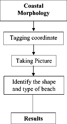
Figure 1.
Collecting Primer Data Flow of Coastal Morphology
The results of processing the average wind speed from ECMWF data for 1991 to 2000 in Figure 2 below. The graph shows the wind speed for a 10 year period
from 1991 to 2000. The wind speed is between 0.2 to 6.2 m/s. Changes in wind speed tend to decrease in the final season of Transition Season 2 (September-November) to West Season (December-February) and increase in Transitional Season 1 (March-May) to East Season in June-August.
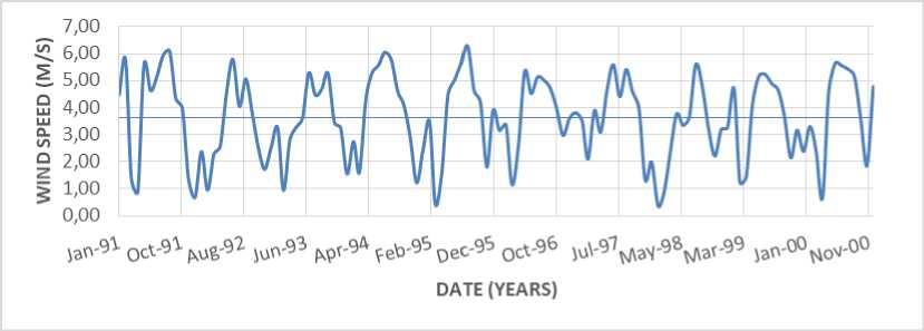
Figure 2.
Wind Speed Rate (1991-2000)
This wind speed graph (in Figure3) shows the wind speed for a period of 10 years from 2001 to 2010. The wind speed is between 0.2 to 6.0 m/s. Changes in wind speed tend to decrease at the end of
the month (September-November) to the month (December-February) and begin to increase around the month (March-May) to June-August.
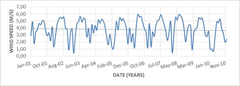
Figure 3.
Wind Speed Rate (2001-2010)
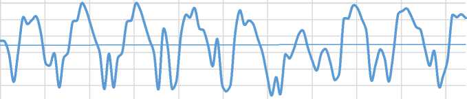
In the west monsoon in December-February, the wind shows gusts of wind originating from the Asian continent towards Australia (Asian Monsoon). While the east monsoon in June-August, the wind shows gusts coming from the Australian continent towards Asia (Australian Monsoon). And the wind speed chart (in Figure 4) shows the wind
speed for a period of 10 years from 2011 to 2019. The wind speed is between 0.3 to 6.1 m/s. Changes in wind speed tend to decrease in the final season of Transition Season 2 (September-November) to West Season (December-February) and increase in Transitional Season 1 (March-May) to East Season in June-August.
7,00
X 6,00
5,00
2 4,00 ⅛ 3,,00 g 2,00 f 1,00
0,00
W^ Ot*'^ ^⅛λ^ juO'^ ^λ4 φ⅛'^ QeC-^ otf∙'^6 W^ vJ∖a'<'^ ^a^
DATE (YEARS)
-
Figure 4.
Wind Speed Rate (2011-2019)
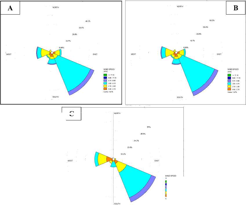
The wind speed describe in Figure 5 below. This windrose shows that the magnitude of the dominant wind speed is between 5.70-8.80 m/s with a percentage of 54.5% and wind speed of 3.60-5.70 m/s with a percentage of 43.6%. The
magnitude of the wind speed in 19811990 was dominant from the Southeast or the Australian continent. The Windrose shows that the magnitude of the dominant wind speed is between 5.70-8.80 m/s with a percentage of 49.3% and wind speed of
-
3.60- 5.70 m/s with a percentage of 39.4%. The lowest wind speed is in the range of 0.50-2.10 m/s. The wind speed in 19811990 was dominant from the Southeast or th
that the magnitude of the dominant wind speed is between 5.70-8.80 m/s with a percentage of 49.3% and wind speed of 3.60-5.70 m/s with a percentage of 39.4%.
C
NORTH
>= 11.10
8.80 -
11.10
- 8.80
5.70
3.60
- 2.10
0.50 -
Calms: 0.96%
WIND SPEED (m/s)
Figure 5.
Windrose (A) 1990-2000; (B) 2000-2010 and (C) 2011-2019
The amount of wind speed in 20012010 was dominant from the Southeast or the Australian continent. This shows that the east monsoon is more dominant than the west monsoons, which generally occur in June-August to September-November. The winds originate from the Australian continent towards Asia (Australian Monsoon). This windrose shows that the wind conditions in the East Season 20112019 are dominated from the Southeast. The winds that occur in this eastern
monsoon are also dominated by dominant wind speeds between 5.70-8.80 m/s with a percentage of 57% and wind speeds of 3.60-5.70 m/s with a percentage of 45.6%. The amount of wind speed in 2011-2019 is predominantly coming from the Southeast or the Australian Continent (Australian Monsoon). This shows that the east monsoon is more dominant than the west monsoon, which generally occurs in June-August.
The DSAS Result in periode I shown in Figure6. In Figure 6a have 3 areas that experience significant shoreline changes. There is Padangbai Village has an average NSM/EPR abrasion value: -116.12 m/-10.19 m/y and accretion of 93.80 m / 8.24 m/y, Bugbug Village has an average NSM/EPR abrasion value: -103.06 m/ -9.05 m/y and accretion of 7.14 m/ 0.63
m/y and East Seraya Village has an average NSM/EPR abrasion of -126.78 m/ -11.13 m/y and accretion of 28.58 m / 2.51 m/y. In Figure 6b above Ketewel Village has an average NSM/EPR abrasion value: -249.56 m / -21.91 m/y and 0 accretion.
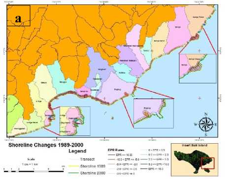
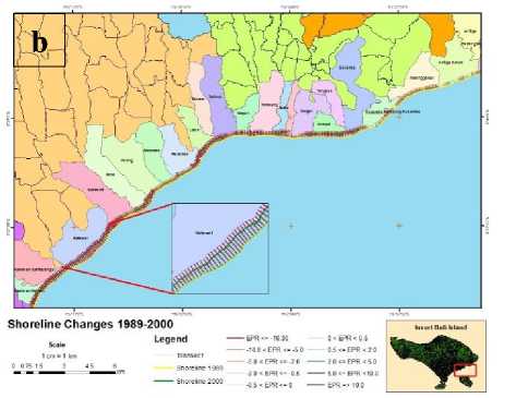
Figure 6.
Shoreline Change 1998-2000
The Figure 7 above shows the difference in the change speed in the shoreline based on the DSAS transect from 1989 to 2000. Four areas experience
a significant rate of change. The area is around Ketewel, Padangbai, Bugbug and East Seraya Villages.
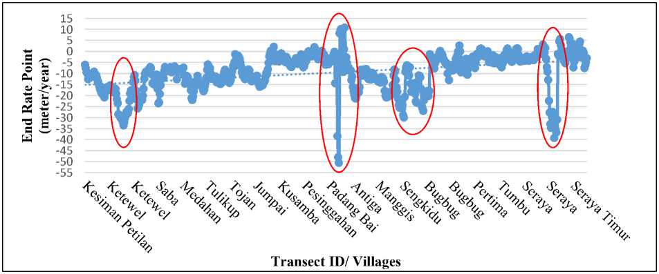
Figure 7.
Dynamical Shoreline Changes (m/y) 1989-2000 by Villages
In Figure 8a three areas experience significant shoreline changes. Padangbai has an average NSM/ EPR abrasion value: -17.29 m/ -1.69 m/y and an accretion of 27.86 m/ 2.72 m/y, Bugbug has an average NSM/ EPR abrasion value: -21.07 m/ -2.06 m/y and an accretion of 23.55 m/ 2.30 m/y, and East Seraya has an average
NSM/ EPR abrasion value of -26.19 m/ -2.55 m/y and accretion of 17.76 m/ 1.73 m/y. And Figure 8b shows area that experienced significant shoreline changes. The Jumpai has an average NSM/ EPR abrasion value: -76.87 m/ -7.50 m/y and accretion 19.51 m/ 1.90 m/y.
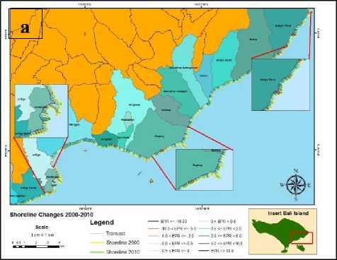
Figure 8.
Shoreline Change 2000-2010
The Figure 9 shows the difference in the speed of change in coastlines based on the DSAS transect from 2000 to 2010. This Figure9 shows the change in the EPR
coastline from 2000 to 2010 based on location per village. This can be used to determine the location of villages that are experiencing high abrasion and accretion.
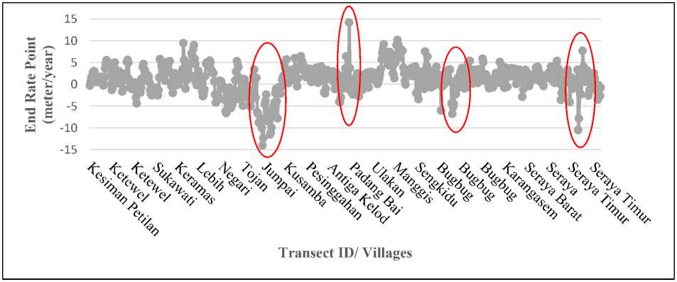
Figure 9.
Dynamical Shoreline Changes (m/y) 2000-2010 by Villages
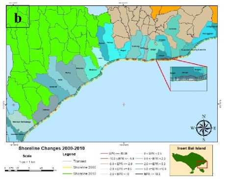
In Figure 10a two areas experience significant shoreline changes. Padangbai has an average NSM/ EPR abrasion value: -18.81 m/ -1.99 m/y and an accretion of 29.13 m/ 3.08 m/y, and Bugbug has an average NSM/ EPR abrasion of -28.38 m/ -3.00 m/y and accretion of 13.14 m/ 1.39 m/y. In Figure10b above two areas
experience significant shoreline changes. The Jumpai has an average NSM/ EPR abrasion value: -48.53 m/ -5.12 m/y and an accretion of 9.73 m/ 1.03 m/y and Gunaksa has an average NSM/ EPR abrasion value: -76.65 m/ -8.09 m/y and accretion 79.48 m / 8.39 m/y.
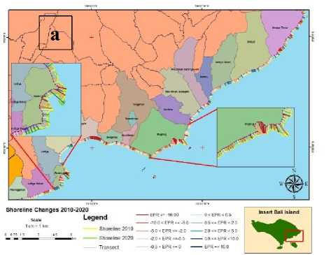
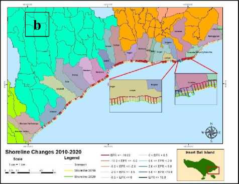
Figure 10.
Shoreline Change 2010-2020
The Figure 11 above shows the difference in the speed of change in coastlines based on the DSAS transect from 2010 to 2020. Three areas have
experienced a significant changes. The area are Gunaksa, Padangbai and Bugbug villages.


20,00
15,00
10,00
5,00
0,00
-5,00
-10,00
-15,00
-20,00
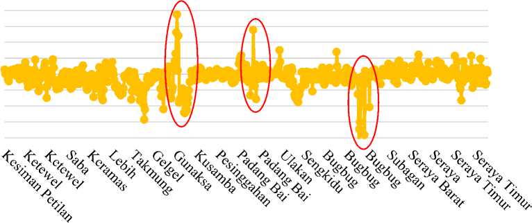
Transect ID/ Villages
Figure 11.
Dynamical Shoreline Changes (m/y) 2010-2020 by Villages
In Figure 12a two areas experience has an average NSM/ EPR abrasion value:
significant shoreline changes. Padangbai -22.72 m/ -5.45 m/y and an accretion of
24.01 m/ 5.75 m/y and Bugbug has an average NSM/ EPR abrasion of -35.40 m/ -8.49 m/y and accretion 23.50 m/ 5.63 m/y. In Figure12b above there is Gunaksa has
an average NSM/ EPR abrasion value: -88.14 m / -21.13 m/y and accretion of 40.74 m/ 9.76 m/y.
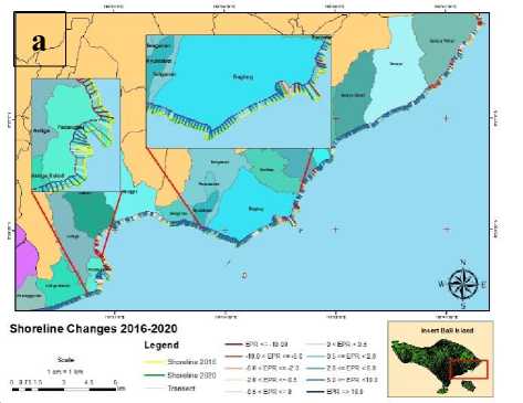
Figure 12.
Shoreline Change 2016-2020
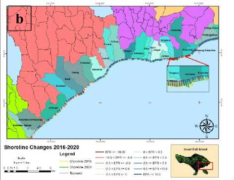
change in the EPR coastline from 2016 to 2020 based on location per village. The Jumpai, padangbai and Bugbus are villages that highly dynamic.
The Figure 13 above shows the difference in the speed of change in coastlines based on the DSAS transect from 2016 to 2020. The graphic shows the
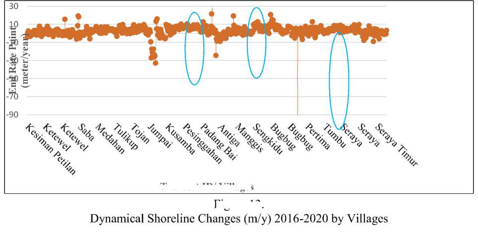
Transect ID/ Villages
Figure 13.
Changes in the coastline in 1989 -2000, the highest level of abrasion occurred in Ketewel, namely -249.56 m with an abrasion rate of -21.91 m/y. The
highest accretion occurred in Padangbai with an average distance of 93.80 m and an average accretion rate of 8.24 m/y. This is made possible by the existence of Padangabai Harbor and jetty around the
Port. The direction of the abrasion movement is the same as the direction of the coming dominant wind from the southeast according to the prediction of the dominant wind direction and speed as described by windrose.
The amount of accretion in this period is greater than in periods II, III and IV. It is possible that the beginning of the construction of the Padangbai Port was possible. (Putra et al, 2015) Pier I Padangbai Port was built in 1994, operated starting in 1997 with a maximum strength of 1,000 gross tonnage (GT). This accretion causes abrasion in other areas due to the dynamic nature of abrasion and accretion and is influenced by wind, waves, rivers, human activities and others.
Based on calculations with DSAS, from the 2000-2010 period, it can be seen that the highest level of abrasion occurred in Jumpai, -76.87 m with an abrasion rate of -7.50 m/y. Meanwhile, Padangbai was the area with the highest accretion of 27.86 m/ 2.72 m/y. This is due to sedimentation in the port due to the harbor building and coast protection. In this period, the accretion and abrasion values were smaller than the previous period. This is possible because there is no offshore development at the port.
The result form 2010-2020, Gunaksa and Jumpai have the highest accretion and abrasion. The highest accretion occurred in Gunaksa, with an average distance of 79.48 m and an average growth rate of 8.39 m/y. This is probably due to the mouth of the Telaga Waja River and Gunaksa Port. Meanwhile, we encountered abrasion of -48.53 m/ -5.12 m/y which was possible due to changes in waves and the result of sedimentation at the mouth of the Telaga Waja river.
And the result from 2016 until 2020, Tangkas and Gunaksa have the highest accretion and abrasion. Gunaksa Village has an average NSM/EPR abrasion value:
-88.14 m/ -21.13 m/y and an accretion of 40.74 m/ 9.76 m/y. The highest level of abrasion occurred in Tangkas, namely -92.82 m with an abrasion rate of -22.24 m/y. The highest accretion occurred in Gunaksa, with an average distance of 40.74 m and an average accretion rate of 9.76 m/y. This is probably due to the mouth of the Telaga Waja River and Gunaksa Port.
Identification of shoreline changes over the past 30 years can be made using the DSAS method using Landsat and Sentinel imagery. This method can also be supported by the prediction of wind speed and wind direction forming seawater waves. In the DSAS method, NSM and EPR values are employed to assess the location/ transect where abrasion occurs (negative) or accretions (positive). The average wind speeds from ECMWF data from three periods 1991-2000; 2001-2010 and 2011-2019 illustrate the dominant wind direction from the Australian continent (southeast). This shows that the east monsoon is more dominant than the west monsoon. In the last 30 years (19892020) the dynamics of shoreline changes can be seen from the EPR graph for each transect which has an average abrasion rate of -6.39 m/y and an accretion rate of 3.15 m/y. The identification results of period I abrasion and accretion areas namely Padangbai and Ketewel have an average abrasion/accretion value of -21.91 m/y (extremely abrasion) and 8.24 m/y (very high); In the period II, namely Jumpai and Padangbai had an average abrasion/accretion value of -7.50 m/y (very high) and 2.72 m/y (high); In period III, namely Jumpai and Gunaksa had an average abrasion/accretion value of -5.12 m/y (very high) and 8.39 m/y (very high).
And in period IV are Tangkas and Gunaksa with an average
abrasion/accretion value of -22.24 m/y (Extremely) and 9.76 m/y (very high).
For further research, the use of other statistical analyzes can be tried by including additional variables such as tide and wave data in order to obtain better results; and Further analysis is needed regarding sediment transport and vulnerability in the Research area
REFERENCE
Arief, Muchlisin, Gathot Winarso, Teguh
Prayogo. 2011. Kajian Perubahan Garis Pantai Menggunakan Data Satelit Landsat di Kabupaten Kendal. Peneliti Pusat Pemanfaatan
Penginderaan Jauh, LAPAN. Jakarta.
Cui B., Li X. (2011) - Coastline change of Yellow River estuary and its response to the sediment and runoff (19762005). Geomorphology, 127: 32-40. doi:
http://dx.doi.org/10.1016/j.geomorph. 2010.12.001.
Fadholi, Akhmad. (2013). Analisis Data
Angin Permukaan Di Bandara Pangkalpinang Menggunakan Metode Windrose. Jurnal Geografi, Media Informasi Pengembangan Ilmu dan Profesi Kegeografian. Semarang University. Semarang.
Istiqomah, F. (2016). Pemantauan
Perubahan Garis Pantai
Menggunakan Aplikasi Digital
Shoreline Anaysis System (DSAS). Studi Kasus: Pesisir Kabupaten
Demak. Jurnal Geodesi Undip. Volume 5, Nomer 1, Tahun 2016.
Kasim, F., 2012. Some Approaching
Methods in Coastline Change Monitoring Using Remote Sensing Dataset of Landsat and GIS.
Agriculture Faculty, Gorontalo University.
Kasim, F., and Aziz Salam. 2015. Identifikasi Perubahan Garis Pantai Menggunakan Citra Satelit serta Korelasinya dengan Penutup Lahan di Sepanjang Pantai Selatan Provinsi Gorontalo. Gorontalo University, Gorontalo. Jurnal Ilmiah Perikanan dan Kelautan. Volume 3, Nomor 4, Desember 2015.
Lakes Environmental. 2013. WRPLOT View-Freeware Wind Rose Plots for Meteorological Data. Cited in https://www.weblakes.com/products/ wrplot/index.html. [19 November 2020].
Luyan Ji, Xiurui Geng, Kang Sun, Yongchao Zhao and Peng Gong. 2015. Target Detection Method for Water Mapping Using Landsat 8 OLI/TIRS Imagery.
www.mdpi.com/journal/water. ISSN 2073-4441.
McFeeters, S.K. 1996. The use of the normalized difference water index (NDWI) in the delineation of open water features. Int. J. Remote Sens. 1996, 17, 1425–1432.
Nugraha, I Nengah Jaya; I Wayan Gede Astawa Karang; I Gusti Bagus Sila Dharma. 2017. Studi Laju Perubahan Garis Pantai di Pesisir Tenggara Bali Menggunakan Citra Satelit Landsat (Studi Kasus Kabupaten Gianyar dan Klungkung). Journal of Marine and Aquatic Sciences 3(2), 204-214
(2017). Bali.
Putra, A., S. Husrin, T.A. Tanto and R. Pratama. (2015). Coastal
Vulnerability for Climate Change in Northeastern Bali Province. Marine Engineering, Bandung Institute of Technology. Available online at www.sciencedirect.com.
Shah, V.P.; Younan, N.H.; King, R.L. 2008. An efficient pan-sharpening method via a combined adaptive PCA
approach and contourlets. IEEE Trans. Geosci. Remote Sens. 2008, 46,
1323–1335.
Sugiarta, eko. 2018. Analisis Perubahan Garis Pantai Menggunakan Citra Satelit Di Pulau Lemukutan, Kabupaten Bengkayang, Kalimantan Barat. Marine and coastal journal, Bogor.
Sun, F.D.; Sun, W.X.; Chen, J.; Gong, P. 2012. Comparison and improvement of methods for identifying waterbodies in remotely sensed imagery. Int. J. Remote Sens. 2012, 33, 6854–6875.
Sutikno, Sigit. (2014). Analisis Laju Abrasi Pantai Pulau Bengkalis dengan Menggunakan Data Satelit Jurusan Teknik Sipil, Fakultas Teknik, Universitas Riau. Riau-Indonesia.
USGS.gov. 2021. Digital Shoreline Analysis System (DSAS). accessed on 9 February 2021 at www.usgs.gov
Xu, H. (2006). Modification of Normalised Difference Water Index (NDWI) to Enhance Open water Features in Remotely Sensed Imagery. International Journal of Remote Sensing, 27(14), 10–12.
74
Discussion and feedback