STUDY ON THE VERTICAL DISTRIBUTION OF CHLOROPHYLL IN COASTAL OCEAN; DEVELOPMENT OF VERTICAL MODEL FUNCTION AT WESTERN SUMBAWA SEA

Written by Nyoman Dati Pertami, Susumu Kanno, I Wayan Arthana
on November 09, 2021

ISSN 1907-5626

Study on the Vertical Distribution of Chlorophyll in Coastal Ocean; Development of Vertical Model Function at Western Sumbawa Sea

STUDY ON THE VERTICAL DISTRIBUTION OF CHLOROPHYLL IN COASTAL OCEAN;

DEVELOPMENT OF VERTICAL MODEL FUNCTION AT WESTERN SUMBAWA SEA

Nyoman Dati Pertami ¹, Susumu Kanno ¹, I Wayan Arthana ²

¹Center for Remote Sensing and Ocean Science (CreSOS), Udayana University

²Master Program of Environmental Study, Post Graduate Program, Udayana University

ABSTRACT

The primary production quantity depends on the vertical distribution of chlorophyll concentration in the water column. The chlorophyll maximum value not always observed near or at the sea surface, but sometimes lies deeper than bottom of the euphotic zone. In this case, the ocean color sensors cannot measure the chlorophyll maximum value. Vertical distribution of chlorophyll modeled and calculated with development of Vertical Model Function (VMF) by “Gaussian function”.

This research has been carried out in western area of Sumbawa Sea. There were 178 stations of field observations. The data were collected at each 0.5 m depth up to 200 m sea depth. Results processing of primary data, with correlations between chlorophyll concentration and depth in every station can show types of vertical distribution of chlorophyll in all stations. There are five types of vertical distribution of chlorophyll at Western Sumbawa Sea. The” five types” then classified into two main groups namely are Linear (L) type and Gaussian (G) type. Finally, data were processed to obtained one especially type that is “one type”. The regression analysis was carried out on the parameters in the Gaussian Function, BO, S, h, σ and Zmax for the each type of the vertical distribution of chlorophyll concentration.

Vertical distribution of chlorophyll found at Western Sumbawa Sea are Linear (L) type, Linear surface (LS) type, Gaussian (G) type, Gaussian with maximum surface (GS) type, and Linear with maximum surface (LMS) type, where with “five types” have nine coefficient determinants (R) which below than 0,25. The regression analysis were modified from “five types” into “two types” and the result was two coefficient determinants (R) that below than 0,25. Correlation coefficient with “one type” have better result than the other types which has only one coefficient determinant (R) that below than 0,25.

Keywords: Vertical distributions, Chlorophyll, Gaussian function.

ABSTRAK

Tingkat kesuburan suatu perairan tergantung pada perkiraan sebaran vertikal dari konsentrasi klorofil di dalam kolom air tersebut. Nilai maksimum klorofil tidak selalu berada didekat atau pada permukaan perairan, tetapi terkadang berada lebih dalam di bawah daerah euphotic. Di lain pihak, sensor ocean color dari satelit tidak dapat menghitung nilai maksimum klorofil yang berada dibawah lapisan permukaan. Dengan pengembangan distribusi vertikal klorofil dari fungsi Gaussian maka dapat diketahui dan dihitung sebaran total biomass klorofil secara vertikal hanya dengan menggunakan data klorofil permukaan.

Data sampling di perairan Barat Laut Sumbawa terdapat 178 station pengamatan. Data diambil tiap 0.5 meter sampai kedalaman 200 meter. Hasil pengolahan data primer, dengan melakukan korelasi diantara konsentrasi klorofil dan kedalaman dari masing-masing stasiun pengamatan maka diperoleh tipe distribusi vertikal klorofil di semua lokasi pengamatan. Terdapat lima type sebaran vertikal konsentrasi klorofil di

perairan Barat Laut Sumbawa. Dari hasil “lima tipe” distribusi yang didapat kemudian diolah ke dalam “dua tipe” utama yaitu: bentuk Lurus dan Gaussian. Terakhir pengolahan data juga dilakukan untuk mendapatkan satu tipe utama yaitu bentuk “satu tipe”. Analisis regresi dilaksanakan pada parameter dari fungsi Gaussian, BO, S, h, s dan Zmax untuk masing-masing jenis dengan distribusi vertikal klorofil.

Distribusi vertikal klorofil yang ditemukan di perairan Sumbawa adalah: bentuk Lurus (Linear type), bentuk Lurus di permukaan (Linear Surface type), bentuk Gaussian (Gaussian type), bentuk Gaussian dengan maksimum di permukaan (Gaussian Surface type), dan bentuk Lurus dengan maksimum di permukaan (Linear Maximum Surface type) dimana sembilan koefisien determinan (R) “lima jenis” nilainya lebih rendah dari 0,25. Analisis dimodifikasi oleh pengelompokan data dari tipe "lima jenis" ke dalam tipe "dua jenis" yang menghasilkan dua koefisien determinan (R) yang lebih rendah dari 0,25. Koefisien korelasi ”Satu jenis” memberikan hasil korelasi lebih baik dibandingkan dengan tipe yang lain yang mana memiliki satu koefisien determinan (R) lebih rendah dari 0,25.

Kata kunci: distribusi vertikal, klorofil, fungsi Gaussian.

INTRODUCTION

Chlorophyll is one of important ecoenvironment parameters. The measurement of chlorophyll concentration in the ocean has a great significance in many subjects, such as ecosystem studies, water quality monitoring, and the marine fishery management. The chlorophyll maximum value cannot be observed near or at the sea surface, but sometimes it lies deeper than the bottom of the eupothic zone. The other hands, ocean color sensor provides the information of the photosynthetic pigment concentration for the upper 22% of the euphotic zone. Therefore, the ocean color sensors cannot measure the chlorophyll maximum value in that zone. Platt et al. (1988) with a Gaussian Distribution Model, which represents the vertical distribution of chlorophyll by four parameters, proposed the solution of that problem. Shifted Gaussian model has been proposed to describe the variation of chlorophyll profile which consists of

four parameters, i.e. background biomass chlorophyll, maximum depth of chlorophyll, total biomass chlorophyll above the background, and thickness or vertical scale of the chlorophyll maximum layer.

The primary production quantity depends on the estimated vertical distribution of chlorophyll concentration in the water column. The vertical distribution patterns of chlorophyll concentration depend on seasons and regions.

This research takes location in East Indonesia, the western sea of Sumbawa Island Sea (Latitude 117º-118º E and Longitude 8º-9º S). Sumbawa has many marine resources, like biological and coastal sources but the most important reason; the focused area that is in Western of Sumbawa Sea has not so many human activities in this area. Therefore, the condition of territorial water is clean enough to analyze when

we compare it with the condition of territorial water around Bali Island (Anonymous, 2002).

The objectives of this research are applied shifted Gaussian distribution (especially Vertical Model Function) to calculate the chlorophyll biomass distribution in coastal ocean at Western Sumbawa Sea.

RESEARCH METHOD

These researches have been carried out in Western area of Sumbawa Sea (Latitude 117º-118º E and Longitude 8º-9º S) around Western coastal area of Sumbawa Island and Moyo Island.

The field observations have been carried out three times, the first on 4^th-11^th September 2005, second on 13^th-20^th November 2005, and the last on 23^rd-27^th April 2006. We use two types dataset in this study. Primary data: obtained by field observation (in-situ data), such as meteorological data (wind speed, wind direction, and air temperature), temperature, salinity, turbidity, chlorophyll, and sigma-T (density). Secondary data: satellite image (ocean color by Aqua/MODIS).

Field Observation (In-situ Data)

Before field observation, prepared and learned about all the instruments that will be used. We determined all the location in every station to get all the data. From Global Positioning System (GPS) we fixed position that needed to observe easily. We take the data in different location; in every station, we settle at least 16 points. From

COMPACT-CTD, we recorded the data. We recorded data from all points that had been set before. We set CTD to record data with depth range every 50 cm. Parameters that recorded by CTD such as temperature, salinity, turbidity, chlorophyll concentration, and sigma-T (density). Echo sounder used to determine the depth of each station by sonic wave.

Transfer Data from CTD to SCV

Daily data recorded from every station of field observation were transferred using Microsoft excel. The first, we converted data recorded by CTD into Comma Separate Value (CSV). Then, we made a graph that shows relationships between depth and temperature or chlorophyll concentration in every station.

Development of Vertical Model Function

Vertical distribution of chlorophyll can be estimated with development of Vertical Model Function (VMF). Shifted-Gaussian model used to represent the chlorophyll vertical profiles and to retrieve five profiles parameters. The model it self is sufficiently versatile to describe a large variety of profiles range from coastal, upwelling, open oceans, and Artic water. The biomass vertical distributions had been determined by applying Gaussian Function (Platt, 1988; Morel, 1989). Shifted Gaussian distribution applied by Gauss parameters as follow (Platt, 1988)

B(Z) = BO + S x Z + h exp [- ( Z – Zmax )² ] δ√2π 2δ²

where :

B(Z) is the chlorophyll concentration (mg.m^-3) at each depth Z (m).

BO is the background chlorophyll concentration at sea surface (mg.m^-3).

S is the vertical gradient of the chlorophyll concentration (mg.m^-3.m^-1).

h is the total chlorophyll above the background (mg.m^-2).

δ standard deviation of Gaussian distribution, which controls the thickness of the chlorophyll maximum layer (m).

Zm is the depth of the chlorophyll maximum (m).

BE

The total biomass can be calculated by ∫ B(Z) dZ

0 where:

- BE is depth at the bottom of euphotic zone.

Data obtained from field observation put into Gaussian function. Then, we determine five parameters in Gaussian Function by empirical regression as show in Figure 2.1.

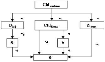
Pioceduic for estimating five parameter from chlorophyll Concentiation at sea surface (⅛_r4J∙Cl⅛._ui≡the maximum chlorophyll concentration at chlorop hyllmaximum layer. *1 Regιpssionas functions of Chlorophyll surface (Chl_lurfwiw); * 2 Regression as functions of B₀ *3 Regiesio nas functions of Chl_xrwu; *4 Calculated by equation as follows,

O=h∕(⅛T( Chl_lmll-B₀-SxZ_mll))

Figure 2.1 Procedure for estimate the five parameters from chlorophyll concentration at sea surface

The five parameters are background biomass chlorophyll (Bo), maximum depth of chlorophyll (Zm), the vertical gradient of the chlorophyll concentration (S), total biomass chlorophyll above the background (h), and thickness or vertical scale of the chlorophyll maximum layer (σ). Then, we crosschecked between in-situ surface chlorophyll and Vertical Model Function. Regression equation to estimate vertical distribution of chlorophyll concentration for the area:

Crosscheck with Observation Data

After steps of the validation about Gaussian function (Vertical Model Function), we crosschecked with in-situ chlorophyll (in-situ observation graph) to know the accuracy of Vertical Model Function.

BO	= A x Chlsurface + B
S	= C x BO + D
ChlZmax	= E x Chl_surf_ace + F
h	= G x ChlZmax+ I
Zmax	= J x Chlsurface+ K

Comparison with Satellite Image

Total biomass of chlorophyll concentration from Vertical Model Function (VMF) compared with ocean color (Aqua/MODIS) satellite image to check the difference among them. If the result between them different we can conclude, that Vertical Model Function which we develop can give additional information for satellite image.

RESULTS AND DISCUSSIONS

The Vertical Distribution of the Chlorophyll Concentration

There are five type vertical distribution of chlorophyll concentration at Western Sumbawa Sea amely are: “Linear (L)” type (Figure 3.1), “Linear surface (LS)” type (Figure 3.2), “Linear with maximum surface (LMS)” type (Figure 3.3), “Gaussian (G)” type (Figure 3.4), and “Gaussian with maximum surface (GS)” type(Figure 3.5).

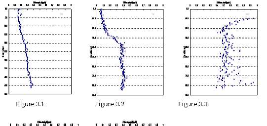
In Gaussian (G) type, the chlorophyll maximum appeared in the mid layer. In Gaussian with surface maximum (GS) type, the chlorophyll maximum is located at or near the sea surface. In Linear (L) type, there is a linear gradient of chlorophyll without prominent peaks. In Linear Surface (LS) type, there is a linear gradient at or near the sea surface but there is higher chlorophyll in the lower layer. The last, in Linear Maximum Surface (LMS) type, there is a maximum of chlorophyll in the surface with linear gradient in mid layer.

Regression Analysis for Parameter Estimation

The vertical distribution of the chlorophyll concentration can be estimated in order five parameters. The regression analysis was carried out on BO, S, h, σ and Zmax for the each type. The grouping of “five types” into “two types” and “one type” modified the regression analysis too.

Correlation coefficients with the “one type” have higher coefficients determinant (R) for each parameter than the other types, where the highest coefficient determinant (R) give advantages in the result as shown in Table 3.1 to 3.3.

Table 3.1 The regression with the five types

EQUATION	R
EQUATION	LS	L	G	GS	LMS
B ∩ Ax Chlsu rf ■» w + B	0.23	0.40	0.50	0.4 1	0.34
Chl_llntl =Ex Chl_surtll,+ F	0.52	0.56	0.29	0.73	0.99
Z_m41 = J X Chl su∣-⅛_cs+ K	0.28	0.34	0.02	0.07	0.18
S = C x B 0 + D	0.24	0.19	0.28	0.13	0.20
h = G x Chl _lm4x + I	0.29	0.04	0.48	0.81	1.00

Table 3.2 The regression with the two types

EQUATION	R
EQUATION	G an s sian	Linear
B∩= A x Chl + B	0.42	0.54
Chl _:„_; = E x Chl _sπ,_ficψ + F	0.41	1 .00
Z_ul,_i = J x Chl + K	0.33	0.37
S = C x B₀ + D	0.1 9	0.1 2
h = G x Chl ^.+ I	0.57	0.99

Table 3.3 The regression with the one tyρe

EQUATION		R
EQUATION		One Type
Bn	= 0.7701 X Chl _lllf,-_i + 3,2741	0.50
C h I z_m	,₁ = 0,9341 X Chl _i,_tfιcf + 0,6828	0.99
^m ax	= -1 ,5169 X Chl _i,_rf,,_ce + 36,975	0.33
S	= 6E-05 XB.-.+ 0,0023	0.08
h	= 99 ,22 X Chl Z_maχ - 58,862	0.99

Correlation between background chlorophyll concentration at sea surface and vertical gradient of the chlorophyll concentration have lower result with “One type” than the other types, because with “one type” data we classification into one group.

Comparison with Surface Chlorophyll from Observation Data

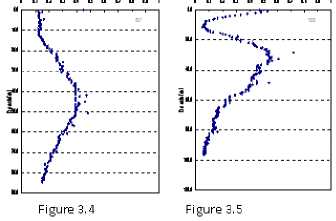
Chlorophyll biomass pattern analyzed by Gaussian Model can give us some useful information which satellite cannot retrieve. Pattern of chlorophyll biomass with the one type can give different pattern around field observation than the other ones. The highest correlation between five parameters might provide more efficient determination of the biomass patterns as shown in Figure 3.6 to 3.8.

Figure 3.6 Chlorophyll biomass pattern obtained by the five types (left) and surface chlorophyll patterns (right) in all observations

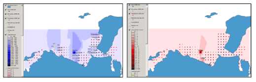
Figure 3.7 Chlorophyll biomass pattern obtained by the two types (left) and surface chlorophyll patterns (right) in all observations

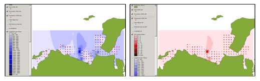
Figure 3.8 Chlorophyll biomass pattern obtained by the one type (left) and surface chlorophyll patterns (right) in all observations

Patterns of Chlorophyll Biomass for Each Observation Period

Gaussian Model can give us information until mid layer by using only surface chlorophyll (Figure 3.9 to 3.10) but surface chlorophyll pattern from ocean color satellite only could give us information from surface layer (Figure 3.11) because ocean color signal is upwelled from surface and the subsurface layer. This means that we can know the biological information in the interior of

Study on the Vertical Distribution of Chlorophyll in Coastal Ocean; Development of Vertical Model Function at Western Sumbawa Sea

ocean by the combination of both Gaussian model and ocean color satellite imagery in a wide spatial

There is a different pattern in periodic,

regional, and seasonal scales. There are significant

differences between the patterns of chlorophyll

coverage.

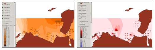
Figure 3.9 Chlorophyll biomass

Fig ure 3.10 Chlorophyll surface in “one type” in first observation

biomass and surface chlorophyll in most of the case

as shown in Figure 3.12 to 3.19.

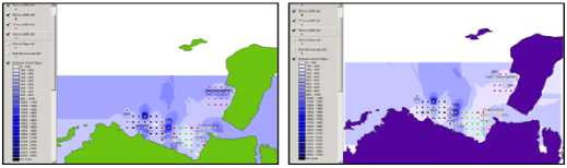
Figure 3.12 Chlorophyll biomass Figure 3.13 Chlorophyll biomass

“five types” in second “two types” in second

observations observations

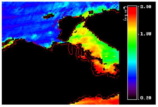
Figure 3.11 Chlorophyll surface pattern by AQUA/MODIS (September 5^th, 2005)

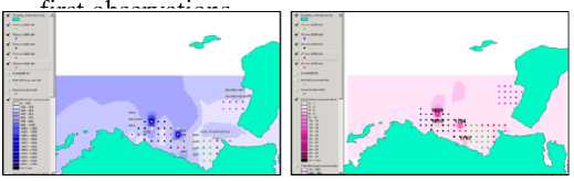
Figure 3.15 Chlorophyll surface in second observations

Figure 3.14 Chlorophyll biomass “one type” in second observations

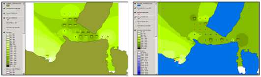
Figure 3.16 Chlorophyll biomass

“five types” in third observations

“two types” in third observations

Figure 3.17 Chlorophyll biomass

Pattern of horizontal gradient, high and low patches of surface chlorophyll do not always match with ones of chlorophyll biomass. In Kameda and Matsumura (1998), seasonal and regional influences on the vertical distribution explained. After we analyzed the data by each type with all period observations, we classified the data with each period of observation.

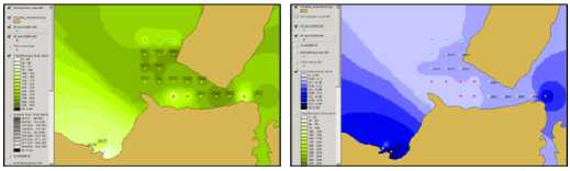
Figure 3.18 Chlorophyll biomass Figure 3.19 Chlorophyll surface in “one type” in third third observations

observations

The Gaussian (G) type is a dominant type than the other ones as shown in Table 6.1. Lalli and Parson (1993) commented on the relationships

between mixing, nutrients and the vertical distribution of phytoplankton in the subsurface layer.

Table 6.1 Number of vertical distribution patterns appeared in each observation

Period of Observation	Numbe r of Station s	TYPE
Period of Observation	Numbe r of Station s	G	GS	L	LS	LMS
4^th – 11^th Sept 2005	75	42	0	19	14	0
13^th – 20^th Nov 2005	77	51	11	1	1	12
23^rd – 27^th April 2006	26	19	1	4	2	0

Then, Sumbawa Sea has clear water, few human activities, and the most important thing is that Sumbawa Sea has accessible strong sunshine into territorial water. The solar light can penetrate into the oceans until depth around 100 to 200 meters. The well-lighted region of the euphotic zone exists between the surface layer and 80 meters, because territorial water of Sumbawa has the strong sunshine and its water is clear to transmit the visible ray into deep zone. Therefore reaction of the photosynthesis take place in the restricted zone of territorial water which is deeper than surface, because sunshine was too strong at the surface.

The transparency of seawater is important to plant life in the ocean and it is a subject of concern to biological oceanographers (Basu, 2003). The transparency of seawater around Sumbawa Sea is over than 20 meters in most of cases. It measures in

terms of the transmission of light introduced artificially in water at depths below the photic zone. The transparency of water in the ocean is quite variable. However, the transparency of Sumbawa Sea is high as explained above. These above facts suggest that the too strong sunshine can not be utilized for photosynthesis in ocean surface, but the intensity of solar radiation is decreased as depth and becomes suite for photosynthesis in somewhere of mid layer. Therefore, the Gaussian type of the vertical distribution appears in most of observation.

Regression analysis of five parameters between vertical gradient of the chlorophyll (S) and background chlorophyll at sea surface (BO) with five, two and one types almost show low coefficient determinant (R) as shown in Table 3.1 to 3.3. However, the most important fact is that the vertical distribution model can be represents by one type of curve.

This simple approximation might be derived from the situation in the observation area such as; relatively small area, location facing to open ocean, high transparency. It expected that these simple and similar conditions of ocean environment make the five types integrate into one type.

CONCLUSION AND SUGGESTION

Conclusions

Development of Vertical Model Function (VMF) at Western Sumbawa Sea can be concluded as follows:

There are five types of the vertical distribution of chlorophyll at Western Sumbawa Sea, namely: Gaussian (G) type, Gaussian with surface maximum (GS) type, Linear (L) type, Linear surface (LS) type, and Linear maximum surface (LMS) type. The Gaussian (G) type is a dominant type at Western Sumbawa Sea.

The regression analysis between five parameters in the Vertical Model Function (VMF) is separate into five, two and one types. Coefficient determinant between five parameters with “one type” have highest result than the other types.

Chlorophyll biomass pattern around station 1704 on November 17, 2005 with each type shows significant pattern than the other observations. Comparison chlorophyll surface and chlorophyll biomass have a similar patterns only around stations 1704 and 1707 on November 2005. However, the other observation location have flat pattern from chlorophyll surface. The significant differences were found between the patterns of chlorophyll biomass and surface chlorophyll in most of the case.

Ocean color satellite can provide only information from surface layer, but Gaussian Model can give us information from surface to mid layer and can provide the information in the interior of ocean with wide spatial coverage when it is combining with satellite data.

Suggestions

Development of Vertical Model Function (VMF) utilized to develop the system to find effective fishing ground for the fish migrating mid layer of the ocean and fishery resource management, since sometimes we can find some useful species of fish in mid layer.

Vertical Model Function (VMF) by the vertical distribution of chlorophyll in coastal area gives us only information with small coverage. In further research, we should expand the research with wide spatial coverage and several different ocean environments to improve the suitability and accuracy of the model. For fishery resource management, the Vertical Model Function can be utilized to find fishing ground from viewpoint of not only efficient catch plan but also the fishing resource preservation by sharing the fishery resource with the correct information of the ocean productivity.

ACKNOWLEDGMENT

The author would like to thank and appreciate to Mr. Ohgane (Zeal ocean office), Mr. Tani (Tetsu-Gumi Underwater Operation Co, Ltd) and Mr. Yanagawa (Kyowa Concrete Ltd. Japan) for their provision of opportunities to have experience in oceanographic observation, their direction, and to staff in CV. Marine Tech for their cooperation.

REFERENCES

Anonymous, 2002. Bali - Lombok – Sumbawa – Komodo Islands – Flores. http://www. Bali-indo.com/lombok/places.htm.

Basu, S.K. 2003. Hand Book of Oceanography. Volume 1. Global Vision Publishing House, 19A/E, G.T.B. Enclave, Delhi-110093. India. Website: global visionpub.com.

Gordon, H.R. and Mc. Cluney. 1979. Remote assessment of ocean color for interpretation of satellite visible imagery. A review. Lecture Notes on Coastal and Estuarine Study (Lecture Notes) Vol.4, Springer Verlag.

Kameda, T. and Matsumura, S. 1998. Chlorophyll Biomass off Sanriku, Northwestern Pacific, Estimated by Ocean Color and Temperature Scanner (OCTS) and Vertical Distribution Model. Journal of Oceanography, Vol. 54, pp. 509 to 516.

Nybbaken, J.W. 1993. Marine Biology: An Ecological Approach. Third Edition. Harper Collins College Publishers.

ECOTROPHIC | VOLUME 1 NO. 2 NOVEMBER 2006

9