A COMPARISON OF TIME-VARYING VOLATILITY OF ISLAMIC AND CONVENTIONAL STOCK MARKETS IN INDONESIA
on
BULETIN
EKONOMI

STUDI

BULETIN STUDI EKONOMI
Available online at https://ojs.unud.ac.id/index.php/bse/index
Vol. 28 No. 02, Agustus 2023, pages: 123-133
ISSN:1410-4628
e-ISSN: 2580-5312

A COMPARISON OF TIME-VARYING VOLATILITY OF ISLAMIC AND CONVENTIONAL STOCK MARKETS IN INDONESIA
Arie Sukma1
Abstract
|
Keywords: |
Using daily data from January 2003 to December 2021, this paper |
|
Time-Varying; Markov-Switching; MS-GARCH; Volatility; |
examines the impact of structural changes on the volatility of Islamic and conventional stocks in Indonesia. Assuming that there are two regimes (regular and turbulence) due to these structural changes and using the MSGARCH model, this paper finds that the volatility of Islamic and conventional stocks in Indonesia has a different pattern based on the regime. The volatility of Islamic and conventional stocks tends to increase during turbulence compared to regular periods. However, the negative effect of domestic shocks is more significant on stock volatility than on foreign shocks. In addition, this study also found that the response of Islamic and Conventional stocks looks different. This finding implies differences in characteristics between Islamic and conventional stocks responding to structural shocks. |
Kata Kunci:
Abstrak
Variasiantarwaktu;
Markov-Switching;
MS-GARCH;
Volatilitas;
Koresponding:
Fakultas Ekonomi dan Bisnis, Universitas Andalas Padang, Sumatera Barat, Indonesia 25163
Email:
Dengan menggunakan data harian mulai dari Januari 2003 hingga Desember 2021, tulisan ini menguji dampak perubahan struktural pada volatilitas saham shariah dan konvensional di Indonesia. Dengan mengasumsikan terdapat dua rezim (normal dan turbulensi) akibat perubahan structural tersebut dan menggunaan model MS-GARCH, tulisan ini menemukan bahwa volatilitas saham syariah dan konvensional di Indonesia memiliki pola yang berbeda berdasarkan regim. Volatilitas saham syariah dan konvensional cenderung meningkat Ketika periode turbulensi dibanding periode biasa. Namun demikian, efek negative guncangan dari dalam negeri lebih besar terhadap volatilitas saham dibanding guncangan luar negeri. Selain itu, penelitian ini juga menemukan bahwa respon saham syariah dan konvensional terlihat berbeda terhadap guncangan. Hal ini mengimplikasikan bahwa terdapat perbedaan karakteristik antara saham syariah dan konvensional dalam merespon perubahan struktural.
Fakultas Ekonomi dan Bisnis, Universitas Andalas Padang, Sumatera Barat, Indonesia 25163 Email: ariesukma@eb.unand.ac.id
INTRODUCTION
The Autoregressive Conditional Heteroskedastic (ARCH) model of Engle (1982) and The Generalized Autoregressive Conditional Heteroskedastic (GARCH) model of (Bollerslev, 1986) are the most popular models for predicting the volatility of an asset's return. Nelson (1991), Glosten et al. (1993), and Zakoian (1994) develop EGARCH, GJRGARCH, and TGARCH to improve the ARCH and GARCH model to capture the existence of the possibility of leverage effect on return volatility. There have been many variations of the ARCH model in analyzing volatility in financial econometrics; among them are iGARCH, apARCH, fGARCH, mcsGARCH, realGARCH, and fiGARCH. For a detailed explanation, see Engle &Bollerslev (1986), Ding et al. (1995), Hentschel (1995), Engle &Sokalska (2012), Hansen et al. (2012), and (Baillie et al., 1996). For the implementation in software like R Package, see (Ghalanos, 2022). The ARCH model was also developed as a multivariate model to see the spillover effect of one asset to another asset (Bollerslev, 1990; Engle & Kroner, 1995; Engle, 2002).
Apart from the models mentioned above, several researchers (Ardia et al., 2018;Ardia et al., 2019; Bauwens et al., 2014;Klaassen, 2002; Marcucci, 2005) also capture the possibility that unconditional volatility can vary over time following certain states or regimes. Using the standard GARCH when the volatility exhibit regime switching will result in biased volatility predictions (Ardia, 2008). Some researchers try to accommodate state or regime changes by allowing ARCH and GARCH parameters to vary between regimes. Because parameter changes between these regimes have a certain probability and follow the Markov process, this method is called Markov Switching GARCH (MSGARCH).
The MS-GARCH model has been widely used in predicting unconditional volatility not only in the stock market but also in other fields such as world oil, cryptocurrencies, commodity prices, and geopolitical risk (Bouteska et al., 2023; Caporale&Zekokh, 2019; Kristjanpoller& Michell, 2018; Lee & Lee, 2022; Liu & Lee, 2021; Shiferaw, 2023; Wang et al., 2021; Wang et al., 2022). Wang et al. (2022) found that the MS-GACRH model has a high degree of accuracy in predicting the volatility of renewable energy stock prices by considering three regimes. Meanwhile, the latest research from Bouteska et al. (2023) also reveals that the MS-GARCH model can predict stock price volatility due to structural changes due to the covid-19 pandemic.
Indonesia has two types of stock markets: the Islamic and the Conventional, which have different characteristics. Understanding these two markets' behavior gives investors essential information in choosing the optimal portfolio allocation. The differences in the characteristics of Islamic and Conventional stocks also allow for differences in the indices responding to structural changes between specific regimes. Only a few studies discuss Islamic and Conventional stock market behavior in responding to regime change. Furthermore, using the Indonesian case, this paper tries to contribute to the financial economics literature by comparing the differences in the response of Islamic and Conventional stocks to regime changes.
This research aims to model Islamic and Conventional stocks in Indonesia, represented by JKII and JKSE, using MS-GARCH. Using observations from 2003 to December 2022, we believe that the MS GARCH model is the best, considering that several events could trigger a structural break in the JKII and JKSE series during this period. In 2003 – 2005, for example, Indonesia was hit by the issue of terrorism, which significantly impacted changes in the return viability of the two indices analyzed. The global financial crisis in the 2008 – 2009 period also affected domestic stocks' stability. Finally, the Covid-19 pandemic significantly impacted price transaction volume and return volatility. Therefore, when we assume that the three major events are periods of turbulence on the stock market in Indonesia and outside of these times are regular periods, then predictions about the volatility and A Comparison of Time-Varying Volatility of Islamic and Conventional Stock Markets in Indonesia, Arie Sukma
risk of JKII and JKSE that do not accommodate these state or regime changes will produce biased predictions.
The study found that the return of JKII and JKSE fluctuations during the increase of Indonesia's security risks in 2003 and 2005, the global financial crisis around 2008-2009, and the Covid-19 pandemic seemed to be higher than fluctuations in regular times. Using the MS-gjrGARCH model, this study succeeded in estimating the difference in the volatility of JKII and JKSE as a function of the two regimes, namely regular and turbulence. The estimation results show that general volatility tends to be higher during crises. However, the domestic security factor is more influential in increasing stock market volatility in Indonesia, both for Islamic and Conventional stocks. Meanwhile, the global financial crisis had little impact on increased volatility. In addition, the pandemic has had a very significant impact in a relatively short time. This finding implies that domestic factors, such as security risk, are robust compared to external factors, such as the global financial crisis, influencing both Islamic and Conventional volatility variations in Indonesia.
RESEARCH METHOD
This study uses data on Islamic and Conventional stock indices in Indonesia, namely JKII and JKSE. The study obtains the JKII dan JKSE from yahoo finance directly using the quantmod package in the R package (Ryan & Ulrich, 2022). The total samples are 4781 observations for JKII and 4790 for JKSE.
The basis of this study's analysis is JKII and JKSE return. This study calculates the return, rt, using the geometric method, namely rt = log Yt — logYt-1. By using the GARCH (1,1) model, the study model the volatility of JKII and JKSE returns as follows:
where rt is the logarithm of return. μ is the expected value of the conditional return, εt is the error term or also known as the mean corrected return, σt2 is the conditional variance, and the values α1 and β1 indicate the ARCH and GARCH parameters. For the conditional variance equation to be positive, the parametersω >0, α1 > 0 and β1 > 0. Furthermore, εt will be considered as a stationary covariance if and only if the value α1 + β1 < 1. The GARCH model (1,1) is re-estimated using the specifications EGARCH (1,1), gjrGARCH (1,1), and TGARCH (1,1) to anticipate the existence of the leverage effect. The choice of order p = q = 1 as the ARCH and GARCH parameters in this study follows (Hansen & Lunde, 2005), which says that GARCH (1,1) is often the best model.
This paper assumes that during the analysis period, the volatility of JKII and JKSE may change according to two regimes, namely regular and turbulence. Increased unconditional volatility caused by several events that can significantly affect changes in volatility, such as a reduction in security risks, the global financial crisis, and the COVID-19 pandemic, characterize the turbulence period. This study uses the GARCH model to accommodate the regime changes, which allows the parameters to vary based on a particular regime by following the Markov process. Generally, this model is known as the Markov Switching GARCH (MS-GARCH).
Following (Ardia et al., 2019), we state the MS-GACRHa model as follows:
yt∖(st = k,lt-1)~'D(0,hk,t,ξk)......................................................................(4)
a https://CRAN.R-project.org/package=MSGARCH
in other words, given the number of regimes, st = kand the information set at time t — 1, the series yt has a continuous distribution with an average of 0, the variance varies based on the number of regimes, hk,t, and other parameters that incorporated in ξk. In this case yt = (JKll,JKSE} and st = k = 2, so hk,t = (hjκsε,1,t, hjκsε,2,t, hjκn,1,t, hjκn,2,t) where hjκsε,1,t is the JKSE variant in the first regime.
Based on the assumption thatst = k = 2, this study defines the transition matrix following the Markov process as follows:
r P1,1 Vy2i
P LP2,1 P2,2i
where p1,2 = P[st = 2∣st-1 = 1] dan p21 = P[st = 1∣st-1 = 2] are the probability of transition from state st-1 = 1 to st = 2 and st-1 = 2 ke st = 1.
Following (Ardia et al., 2019), the application of the Markov process to the standard model GARCH, eGARCH, gjrGARCH, and tGARCh are as follows:
hk,t = a0,k + a1,kyt-1 + βkhk,t-1(5)
ln(hk,t) = ao,k + a1,k(∣lk,t-1∣ - E[IPk,t-1W) + a2,kPk,t-1+βkln(hk,t-1)
hk,t = Uo,k + (U1,k + a2,kKyt-1 < 0))y2-1+βkhk,t-1(7)
hk^ = a0,k + (a1,k^{yt-1 ≥ 0} - a2,k^(yt-1 < 0})yt-1 + βkhkt-1
where k = 2, in the GACRH standard model, the assumption of positivity is fulfilled by a0,k > 0, a1,k > 0, meanwhile the assumption of stationarity is fulfilled by, a1,k + βk < 1. The eGARCH model specification automatically fulfills the assumptions of positivity and stationarity, requiring βk < 1. For the conditional variance to be positive in the gjrGARCH model, then a0,k > 0, a1,k > 0, 1
a2,k ≥ 0, βk ≥ 0, and the assumption of stationarity requires a1,k + aa2+ + βk < 1. The tGARCH model requires a0,k > 0, a1,k > 0, a2,k > 0, βk ≥ 0 to fulfill the positivity assumption and a2,k + βk - 2 ^βk(al,k + a2,k) — √1 (a¾,k + a2,k) < 1 to satisfy the stationarity assumption.
RESULTS AND DISCUSSION
Table 1 explains the descriptive statistics of JKII and JKSE returns. The samples for JKII are 4781 units and 4790 units for JKSE. On average, the JKSE return of 0.0005 looks higher than the JKII return of 0.0004, but the difference is not too significant. Even the standard deviation of JKSE returns is also slightly lower than JKII. The return of JKII and JKSE also show negative skewness values, indicating an asymmetric distribution for the two returns. In other words, a negative slope indicates the possibility of a return with a negative value being more significant than a return with a positive value. The kurtosis value is also relatively high for both observed indices. A high kurtosis value indicates that there were high return fluctuations in the previous period and are further away from the average value. The risk of this kurtosis depends on the value of the slant. If the slope is positive, then there is a possibility that the return will fluctuate at a higher level. Conversely, if the slope value is negative, the chance of getting a lower return will be greater due to the high kurtosis value (Afzal et al., 2021).
Table 1.
Descriptive statistics of return of JKII and JKSE
|
JKII |
JKSE | |
|
Observations |
4781 |
4790 |
|
Minimum |
-0.1538 |
-0.1131 |
|
Arithmetic Mean |
0.0004 |
0.0005 |
|
Maximum |
0.1205 |
0.0970 |
|
Variance |
0.0002 |
0.0002 |
|
Standard deviation |
0.0152 |
0.0127 |
|
Skewness |
-0.4969 |
-0.6139 |
|
Kurtosis |
7.1376 |
8.1413 |
Source: Author's calculation
-
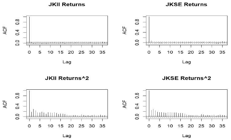
Figure 1 shows the autocorrelation function return and return squared for both indexes. The ACF values of JKII and JKSE returns are each not significant at the 5% level. Almost all bar charts are colored black within the upper and lower limits of blue. Of the 35 lags used for all indices, only 1 or 2 are outside the blue dotted line. In addition, although several bar charts are still outside the boundary line, no specific pattern is detected, indicating a serial correlation. In other words, the number of bar charts outside the boundary line occurs at a random lag, meaning there is no serial correlation (autocorrelation) of all observed returns. The second row in Figure 1 shows the squared return autocorrelation value. All the black bar charts are outside the boundaries of the blue line and show a pattern where ACF is high at the initial lag and continues to decrease at increasing lags. The pattern shows the existence of a serial correlation on quadratic returns. Thus, volatility modeling is better using the GARCH model.
-
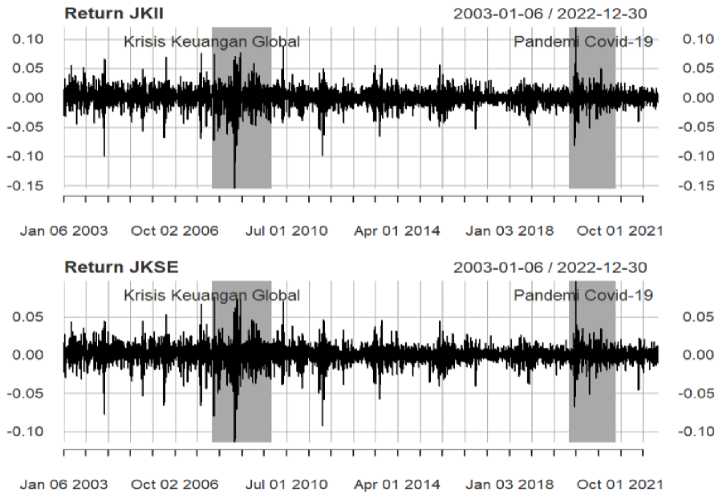
Figure 2 shows that fluctuations in returns for all indices show volatility clustering, where low returns in the previous period tend to be followed by low returns in the following period and vice versa. It is clear that fluctuations of JKII and JKSE return in 2003 and 2005 indicated increased security risks in Indonesia during the global financial crisis around 2008-2009, and the Covid-19 pandemic seemed to be higher than fluctuations during regular times. The data also shows that there are time-varying variations in return volatility. In addition, Figure 2 clearly shows the existence of several outliers, especially in 2003 and 2005, during the global financial crisis and the Covid-19 pandemic. For both series, during the global financial crisis, one data point was quite far from the average of all data with a negative value.
An outlier during the pandemic was quite far from the average return but with a positive value. The phenomenon of volatility clustering and the emergence of outliers in the JKII and JKSE series during the observation period showed variations in conditional variance based on specific regimes (Ardia et al., 2019). This study uses MS-GARCH to model the JKII and JKSE conditional variance series to accommodate variations based on these regimes.
Before using the MS-GARCH model, this study estimates the JKII and JKSE series using the standard GARCH model to determine the best GARCH specification. Table 2 shows the GARCH (1,1) estimates for each index. The α parameter shows the ARCH coefficient, while the β parameter shows the GARCH coefficient. Parameters α and β have positive signs and are significant at the 1% level, as expected. For both indices, the parameter α + β is positive and less than 1, indicating stationarity in returns. The Ljung-Box Test on Lag 1 Standardized Squared Residuals has a p-value > 0.05, meaning there is no reason to reject H_0, that there is no indication of autocorrelation in the model. The ARCH effect no longer exists for all indices. The Nyblom stability test, providing information about structural changes in the index and significant at the 1% level, implies that the estimated parameters vary according to a particular pattern of structural changes (time-varying
127 e-ISSN: 2580-5312 volatility). Furthermore, the sign bias test also shows a significant sign which implies that the index volatility is asymmetric.
Source: Author's calculation
Figure 1.
ACF of returnandsquaredreturnof JKII and JKSE
Source: Author's calculation
Figure 2.
Return of JKII and JKSE
Table 2.
The result of the GARCH model
|
JKII |
JKSE | |
|
μ |
0.0005** |
0.0007** |
|
(0.0001) |
(0.0001) | |
|
ω |
0.0000* |
0.0000* |
|
(0.0000) |
(0.0000) | |
|
α |
0.0987** |
0.1238** |
|
(0.0082) |
(0.0102) | |
|
β |
0.8820** |
0.8533** |
|
(0.0108) |
(0.0145) | |
|
α + β |
0.9796 |
0.9799 |
|
Ljung-Box Test (Lag 1 Standardized Squared Residuals) |
0.5332 |
0.7901 |
|
[0.4652] |
[0.3741] | |
|
ARCH LM Test |
0.9643 |
1.2300 |
|
[0.3261] |
[0.2675] | |
|
Nyblom Test (Join Statistics) |
2.5710** |
3.6670** |
|
Sign Bias Test (t-test) |
1.9540* |
1.7960* |
**Significant at 1%, *Significant at 5%, ( ) standard error, [ ] p-value Source: Author's calculation
The Nyblom test and sign bias in table 2 implies that volatility modeling for both indices needs to accommodate asymmetric and time-to-time variations. Thus, the best way to model JKII dan JKSE volatility is using MS-GARCH with several alternative specifications such as eGARCH, gjrGARCH, and tGARCH. As previously explained, MS-GARCH can explain variations in volatility based on specific regimes, while alternative specifications eGARCH, gjrGARCH, and tGARCH can accommodate asymmetric volatility (leverage effect).
Table 3 describes the MS-GARCH estimation results using three alternative specifications. The gjrGARCH specification must meet the assumptions of positivity and stationarity. Meanwhile, the eGARCh and tGARCH specifications are sufficient to fulfill the assumption of stationarity. The estimation results show that the specifications for the gjrGARCH model for both series meet the assumptions of positivity and stationarity. All estimation parameters are positive for both JKII and JKSE. The gjrGACRH specification also shows covariance stationarity where the value a1,k + a2,k + 1
- βk<1 where k = 2 indicates the number of regimes. In addition, all parameters are also significant at the 1% level. In the eGARCH specification, the study satisfies the stationarity assumption because the parameter values β1 and β2 are smaller than 1 for both series. Next, the tGARCH specification satisfies the assumptions of positivity and stationarity as indicated by the positive values of all estimation parameters and the value a¾,k + βk - 2√^βk(a1,k + α2,k) — √^ (a2k + a2,k) < 1. Model selection refers to the AIC and BIC values, which indicate that gjrGARCh is the best model because it has the smallest AIC and BIC values. Therefore, the gjrGARCH model will infer the volatility of the JKII and JKSE indices.
The MS-gjrGARCH estimation shows that the unconditional volatility of JKII and JKSE looks different based on the regime. In the JKII series, the first and second regimes show a volatility value of 0.21 and 0.25, respectively. In comparison, the first and second regimes in the JKSE series show volatility values of 0.16 and 0.23, respectively. The difference in volatility between regimes seems less significant for the JKII series than for the JKSE, implying that the unconditional volatility of Islamic
stock indexes looks more stable than conventional stocks. However, the unconditional volatility of Islamic looks higher than Conventional stocks.
In the JKII series, the parameters α2,1 and α2,2 that indicate the magnitude of the leverage effect between regimes also has different values. The leverage effect in the first regime is 0.0792, which is smaller than the second regime, which is 0.3709. The same thing is true for JKSE, where the leverage effect in regime 1 is 0.1100, which is smaller than the second regime, which is 0.4689. Based on the index, it turns out that JKSE had a more significant reaction to negative returns in the previous period than JKII. This condition indicates that conventional stocks are more vulnerable to negative publicity than Islamic stocks. In addition, each index also has different persistent volatility between 1
regimes. In the JKII series, the persistent volatility in the first regime is a1,1 + -α2,1 + β1 = 0.98, and 1
the persistent volatility in the second regime is α1,2 + -a2,2 + β2 = 0.79. For the JKSE series, persistent volatility in the first and second regimes is 0.98 and 0.77. In general, the first regime describes a more conducive market situation than the second regime, characterized by relatively low unconditional volatility and weak reactions to negative returns in the previous period but with more persistent volatility. This pattern is almost similar for both series.
Figure 3 further confirms the results obtained in table 3. The top and bottom sections in Figure 3 explain the smoothed probability in the first and second regimes. Around the period from 2003 to 2005, the probability for JKII to be in the first regime (conducive period) is relatively low. The low probability of JKII volatility being in a regular period is due to increased Indonesian security risks during this period. From 2003 to 2005, there were at least two significant incidents, namely the bombings in the Mega Kuningan area and the II Bali Bombing. After 2005, JKII's volatility was more stable, as indicated by the increasing probability that JKII's volatility was in the first regime. One of the exciting things from this study is that during the early period of the global financial crisis, the movement of JKII volatility seemed more stable but did not last for a long time because approaching 2010, the probability of being in the first regime (conducive period) again decreased significantly due to the impact of the global financial crisis in the 2008 and 2009 periods. This illustrates that JKII was only affected during the final period of the global financial crisis. Immediately after the global financial crisis ended, the probability of JKII's volatility returning to a conducive state increased until 2020. Entering the end of the first quarter of 2020, as the Covid-19 pandemic escalated, the probability of JKII moving to the second regime decreased again with an increasing probability of being in the second regime.
Similar results are also valid for JKSE's volatility in responding to security conditions in Indonesia, changes due to the global financial crisis, and the covid-19 pandemic. During the period from 2003 to the end of 2007, along with increasing security risks, the movement of JKSE volatility was relatively stable in the second regime. Likewise, the impact of the global financial crisis was felt by JKSE when it entered the final period of the crisis. After that, JKSE volatility seemed stable in the first regime until it moved back to the second regime due to the co-19 pandemic. However, in general, the probability that JKII and JKSE are in the first regime is 62% higher than the possibility in the second regime, which equals 32%. The results of this study support the previous findings of (Bouteska et al., 2023), which claim that stock volatility reacts significantly to natural calamities.
Table 3.
The result of various estimation methods
|
MS-GJRGARCH |
MS-EGARCH |
MS-TGARCH | ||||
|
JKII |
JKSE |
JKII |
JKSE |
JKII |
JKSE | |
|
alpha0_1 |
0.0000** |
0.0000** |
-0.3802** |
-0.0075* |
0.0001 |
0.0000** |
|
(0.0000) |
(0.0000) |
(0.0245) |
(0.0048) |
(0.0005) |
(0.0000) | |
|
alpha1_1 |
0.0383** |
0.0344** |
0.1137** |
0.1287** |
0.0446** |
0.0315** |
|
(0.0142) |
(0.0131) |
(0.0304) |
(0.0338) |
(0.0161) |
(0.0000) | |
|
alpha2_1 |
0.0792** |
0.1100** |
-0.0663** |
-0.1040** |
0.0656 |
0.0228** |
|
(0.0207) |
(0.0210) |
(0.0146) |
(0.0135) |
(0.2352) |
(0.0000) | |
|
beta_1 |
0.9048** |
0.8878** |
0.9582** |
0.9761** |
0.9447** |
0.9786** |
|
(0.0142) |
(0.0168) |
(0.0025) |
(0.0048) |
(0.1277) |
(0.0000) | |
|
nu_1 |
7.2572** |
6.8615** |
11.6443** |
6.6342** |
7.3451** |
6.1621** |
|
(0.7194) |
(0.6335) |
(1.0478) |
(0.5815) |
(1.2816) |
(0.0000) | |
|
alpha0_2 |
0.0001** |
0.0000** |
-0.7669** |
0.1149** |
0.0020 |
0.0032** |
|
(0.0000) |
(0.0000) |
(0.2937) |
(0.0339) |
(0.0035) |
(0.0000) | |
|
alpha1_2 |
0.0001** |
0.0000** |
0.1095** |
0.3018** |
0.0000 |
0.0000** |
|
(0.0057) |
(0.0005) |
(0.0691) |
(0.0429) |
(0.0001) |
(0.0000) | |
|
alpha2_2 |
0.3709** |
0.4689** |
-0.1907** |
-0.2106** |
0.2529** |
0.1754** |
|
(0.0773) |
(0.0901) |
(0.0366) |
(0.0414) |
(0.1314) |
(0.0000) | |
|
beta_2 |
0.5998** |
0.5389** |
0.8965** |
0.8162** |
0.7843** |
0.7897** |
|
(0.0689) |
(0.0656) |
(0.0385) |
(0.0554) |
(0.2361) |
(0.0000) | |
|
P_1_1 |
0.9980** |
0.9988** |
0.9849** |
0.9987** |
0.9927** |
0.9803** |
|
(0.0018) |
(0.0007) |
(0.0017) |
(0.0003) |
(0.0203) |
(0.0000) | |
|
P_2_1 |
0.0032** |
0.0018** |
0.0656** |
0.0026** |
0.0091 |
0.0857** |
|
(0.0028) |
(0.0012) |
(0.0074) |
(0.0011) |
(0.0113) |
(0.0000) | |
|
Stable probability state 1 |
0.6194 |
0.6091 |
0.8129 |
0.6670 |
0.5561 |
0.8132 |
|
Stable probability state 2 |
0.3806 |
0.3909 |
0.1871 |
0.3330 |
0.4439 |
0.1868 |
|
Unconditional volatility State 1 | ||||||
|
Unconditional volatility State 2 | ||||||
|
AIC |
-28029.3 |
-30176.3 |
-27992.9 |
13946.94 |
-28021.5 |
-29964.2 |
|
BIC |
-27958.1 |
-30105.0 |
-27921.7 |
14018.16 |
-27950.3 |
-29892.9 |
*Significant at 5%, **Significant at 1%, ( ) standard error
Source: Author's calculation
The robustness test of the model aims to see the consistency of the estimation of JKII and JKSE volatility generated by the MS-gjrGARCH specification. In testing the model's robustness, the study uses closing prices and reduces initial and final observations by 100 observations each in calculating JKII and JKSE returns. All procedures for testing the model's robustness are carried out the same way as the previous estimation. Table 4 reports that the results of the robustness test estimation are consistent with this study's previous findings. In addition, Figure 4 also shows the transition probabilities of JKII and JKSE, which are also consistent with the previous ones.
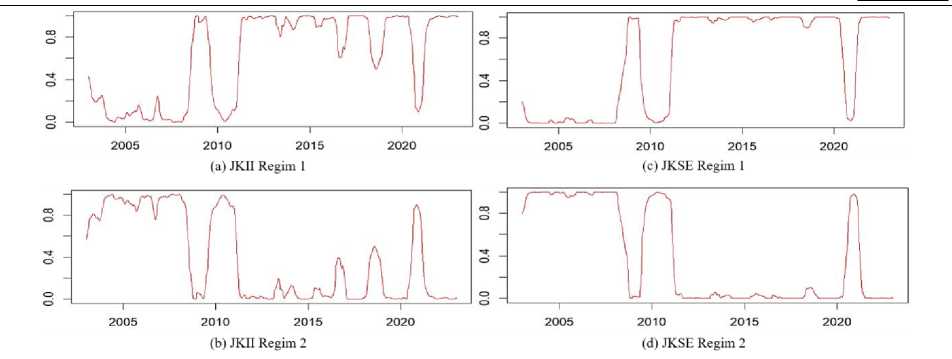
Source: Author's calculation
Figure3.Transition probability of JKII and JKSE across regime
Table4.
The result of the robustness test
MS-gjrGARCH
|
JKII |
JKSE | |
|
Unconditional volatility state 1 |
0.21 |
0.17 |
|
Unconditional volatility state 2 |
0.25 |
0.23 |
|
leverage effect State 1 |
0.07 |
0.11 |
|
leverage effect State 2 |
0.38 |
0.48 |
|
Volatility Persistence State 1 |
0.98 |
0.98 |
|
Volatility Persistence State 1 |
0.78 |
0.78 |
|
Stable probability state 1 |
0.63 |
0.60 |
|
Stable probability state 2 |
0.37 |
0.40 |
Source: Author's calculation
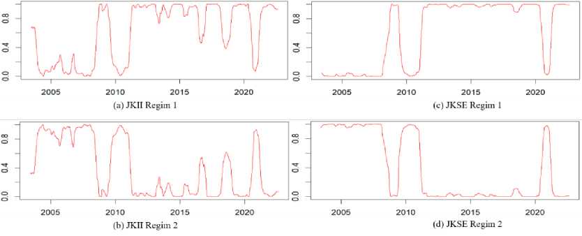
Source: Author's calculation
Figure4.Robustness test of transition probability of JKII and JKSE across regime
CONCLUSION AND SUGGESTION
The study found that the volatility of return's JKII and JKSE is higher due to changes in Indonesia's security risks in 2003 and 2005, the global financial crisis around 2008 – 2009, and Covid-19. Using the MS-gjrGARCH model, this study estimates the difference in volatility of JKII and JKSE based on two regimes, regular and turbulence. The estimation results show that volatility tends to be higher during turbulence. However, domestic security factors have more influence on the increase in stock market volatility in Indonesia, both for Islamic and conventional stocks. Meanwhile, the global financial crisis had little impact on increased volatility. Furthermore, the pandemic significantly impacts in a relatively short time. This finding implies that domestic factors than external factors, such as the global financial crisis, have a more significant influence on both Islamic and Conventional stock volatility in Indonesia.
REFERENCE
Afzal, F., Haiying, P., Afzal, F., Mahmood, A., & Ikram, A. (2021). Value-at-Risk Analysis for Measuring Stochastic Volatility of Stock Returns: Using GARCH-Based Dynamic Conditional Correlation Model. SAGE Open, 11(1). https://doi.org/10.1177/21582440211005758
Ardia, D. (2008). Financial risk management with Bayesian estimation of GRAPH models: Theory and application. In Lecture Notes in Economics and Mathematical Systems (Vol. 612).
Ardia, D., Bluteau, K., Boudt, K., & Catania, L. (2018). Forecasting risk with Markov-switching GARCH models: A large-scale performance study. International Journal of Forecasting, 34(4), 733–747. https://doi.org/10.1016/j.ijforecast.2018.05.004
Ardia, D., Bluteau, K., Boudt, K., Catania, L., & Trottier, D. A. (2019). Markov-switching GARCH models in R: The MSGARCH package. Journal of Statistical Software, 91(4).
https://doi.org/10.18637/jss.v091.i04
Ardia, D., Bluteau, K., & Rüede, M. (2019). Regime changes in Bitcoin GARCH volatility dynamics. Finance Research Letters, 29(July 2018), 266–271. https://doi.org/10.1016/j.frl.2018.08.009
Baillie, R. T., Bollerslev, T., & Mikkelsen, H. O. (1996). Fractionally integrated generalized autoregressive conditional heteroskedasticity. Journal of Econometrics, 74(1), 3–30. https://doi.org/10.1016/S0304-4076(95)01749-6
Bauwens, L., Dufays, A., & Rombouts, J. V. K. (2014). Marginal likelihood for Markov-switching and changepoint GARCH models. Journal of Econometrics, 178(PART 3), 508–522.
https://doi.org/10.1016/j.jeconom.2013.08.017
Bollerslev, T. (1986). Generalized autoregressive conditional heteroskedasticity. Journal of Econometrics, 31(3), 307–327.
Bollerslev, T. (1990). Modeling the Coherence in Short Run Nominal Exchange Rates: A Multivariate Generalized ARCH Model, The Review of Economics and Statistics, 72 (1990), pp. 498–505.
Bouteska, A., Sharif, T., & Zoynul, M. (2023). Research in International Business and Finance COVID-19 and stock returns: Evidence from the Markov switching dependence approach. Research in International Business and Finance, 64, 101882. https://doi.org/10.1016/j.ribaf.2023.101882
Caporale, G. M., & Zekokh, T. (2019). Modeling volatility of cryptocurrencies using Markov-Switching GARCH models. Research in International Business and Finance, 48(July 2018), 143–155.
https://doi.org/10.1016/j.ribaf.2018.12.009
Ding, Zhuanxin, Granger, C. W. J., & Engle, F. (1995). A long memory property of stock market returns and a new model. Journal of Empirical Finance, 2(1), 98. https://doi.org/10.1016/0927-5398(95)90049-7
Engle, R. F. (2002). Dynamic conditional correlation: A simple class of multivariate generalized autoregressive conditional heteroskedasticity models. Journal of Business and Economic Statistics, 20(3), 339–350. https://doi.org/10.1198/073500102288618487
Engle, R. F. (1982). Autoregressive Conditional Heteroscedasticity with Estimates of the Variance of United Kingdom Inflation. Econometrica, 50(4), 987. https://doi.org/10.2307/1912773
Engle, R. F., & Bollerslev, T. (1986). Modelling the persistence of conditional variances. Econometric Reviews, 5(1), 1–50. https://doi.org/10.1080/07474938608800095
Engle, R. F., & Kroner, K. F. (1995). Multivariate simultaneous generalized arch. Econometric Theory, 11(1), 122–150. https://doi.org/10.1017/S0266466600009063
Engle, R. F., & Sokalska, M. E. (2012). Forecasting intraday volatility in the US equity market. Multiplicative component GARCH. Journal of Financial Econometrics, 10(1), 54–83.
https://doi.org/10.1093/jjfinec/nbr005
Ghalanos, A. (2022). Rugarch: Univariate GARCH models. R package version 1.4-8.
Glosten, L. R., Jagannathan, R., & Runkle, D. E. (1993). On the Relation between the Expected Value and the Volatility of the Nominal Excess Return on Stocks. The Journal of Finance, 48(5), 1779–1801. https://doi.org/10.1111/j.1540-6261.1993.tb05128.x
Hansen, P. R, Huang, Z., & Shek, H. S. Realized garch: a joint model for returns and realized measures of volatility. Journal of Applied Econometrics, 27(6):877–906, 2012.
Hansen, P. R., & Lunde, A. (2005). A forecast comparison of volatility models: Does anything beat a GARCH(1,1)? Journal of Applied Econometrics, 20(7), 873–889. https://doi.org/10.1002/jae.800
Hentschel, L. (1995). All in the family Nesting symmetric and asymmetric GARCH models. Journal of Financial Economics, 39(1), 71–104. https://doi.org/10.1016/0304-405X(94)00821-H
Klaassen, F. (2002). EMPIRICAL Improving GARCH volatility forecasts with regime- switching GARCH. 363– 394.
Kristjanpoller R., W., & Michell V., K. (2018). A stock market risk forecasting model through integration of switching regime, ANFIS and GARCH techniques. Applied Soft Computing Journal, 67, 106–116. https://doi.org/10.1016/j.asoc.2018.02.055
Lee, H. T., & Lee, C. C. (2022). A regime-switching real-time copula GARCH model for optimal futures hedging. International Review of Financial Analysis, 84(March), 102395.
https://doi.org/10.1016/j.irfa.2022.102395
Liu, M., & Lee, C. C. (2021). Capturing the dynamics of the China crude oil futures: Markov switching, comovement, and volatility forecasting. Energy Economics, 103(October), 105622.
https://doi.org/10.1016/j.eneco.2021.105622
Marcucci, J. (2005). Studies in Nonlinear Dynamics & Econometrics Forecasting Stock Market Volatility with Forecasting Stock Market Volatility with Regime-Switching GARCH Models. 9(4).
Nelson, D. B. Conditional heteroskedasticity in asset returns: A new approach. Econometrica, 59(2):347–70, 1991.
Ryan J, A, & Ulrich J, M. (2022). _quantmod: Quantitative Financial Modelling Framework_. R package version 0.4.20, https://CRAN.R-project.org/package=quantmod.
Shiferaw, Y. A. (2023). An analysis of East African tea crop prices using the MCMC approach to estimate volatility and forecast the in-sample value-at-risk. Scientific African, 19, e01442.
https://doi.org/10.1016/j.sciaf.2022.e01442
Wang, L., Ma, F., Hao, J., & Gao, X. (2021). Forecasting crude oil volatility with geopolitical risk: Do timevarying switching probabilities play a role? International Review of Financial Analysis, 76(February), 101756. https://doi.org/10.1016/j.irfa.2021.101756
Wang, L., Wu, J., Cao, Y., & Hong, Y. (2022). Forecasting renewable energy stock volatility using short and long-term Markov switching GARCH-MIDAS models: Either, neither or both? Energy Economics, 111, 106056. https://doi.org/10.1016/J.ENECO.2022.106056
Zakoian, J. M. (1994). Threshold heteroskedastic models. Journal of Economic Dynamics and Control, 18(5), 931–955. https://doi.org/10.1016/0165-1889(94)90039-6
A Comparison of Time-Varying Volatility of Islamic and Conventional Stock Markets in Indonesia,
Arie Sukma
Discussion and feedback