Soil Electrical Conductivity (Ec) Mapping Using Real-Time Soil Sensor
on
Jurnal Ilmiah Teknologi Pertanian AGROTECHNO
Volume 5, Nomor 1, April 2020
ISSN: 2503-0523 ■ e-ISSN: 2548-8023
Soil Electrical Conductivity (Ec) Mapping Using Real-Time Soil Sensor
Ni Nyoman Sulastri*, Sakae Shibusawa**, Masakazu Kodaira**
*Faculty of Agricultural Technology, Udayana University, Badung, Bali, Indonesia
**Laboratory of Environmental and Agricultural System, Tokyo University of Agriculture and Technology, Tokyo, Japan
*email: sulastri@unud.ac.id
Abstract
The development of soil electrical conductivity (EC) recently to generate soil EC spatial variability map is increasingly attractive because of its application for site-specific crop management. Several commercial applications have been developed and marketed. The purpose of this paper is to compare soil EC spatial variability map produced by capacitance and spectroscopic sensors. The two sensors (capacitance and spectroscopic sensors) was mounted in a Real-time soil sensor. The spectrophotometer was used that has linearly arrayed photodiodes of 256 channels for 400 to 900 nm for visible (Vis) lights and 128 channels for 900 to 1700 nm for near infrared (NIR) lights. For two capacitance sensors were embedded in soil penetrator (front/ECF and side/ ECS), which its tip with a flat plane edge to make uniform soil cuts and the soil flattener behind produced a uniform surface texture. It was found that spectroscopic method performed better compared to capacitance sensor. Using linear regression, the spectroscopic method has shown a correlation of 0.75 with soil EC generated from laboratory analysis (ECL). While, the capacitance method shows significant different compared to soil ECL. The primary cause of the extreme differences between ECL, ECF and ECS values is likely related to the calibration of the capacitance sensor itself.
Keywords: soil electrical conductivity, spatial variability, on the go soil sensor, precision agriculture, capacitance sensor.
INTRODUCTION
Soil maps, describing the variability of soil within fields, are essential in an integrated precision agriculture system. For that reason, the mapping of soil electrical conductivity (EC) has become a popular practice because of its feasibility and convenience, as it can indirectly identify some physical and chemical properties of soil which may relate to yield variability. An on-the-go soil sensor, also known as a real time soil sensor (RTSS), has been developed and enabled to show the variability of soil EC, moisture content (MC), soil organic matter (SOM), nitrate-nitrogen (NO3-N), total nitrogen (TN), total carbon (TC) and acidity (pH) (Shibusawa et al., 1999). The RTSS collects soil reflectance and soil capacitance data at any depth between 0.15 and 0.35m and is comprised of two types of soil EC sensors, a visible/near-Infrared spectrophotometer (Vis-NIR) and an electrical conductivity sensor installed on the chisel penetrator.
Soil EC sensors that mounted for on-the-go soil
sensor have been commercialized. Buchleaiter and Fahrani (2002), Fritz et al (1999) and Sudduth et al (2003) compared non-contact and contact sensors for mapping soil spatial variability. The studies show similarities spectroscopic and capacitance methods were compared in this study because: (1) no evidence of prior studies comparing spectroscopic and capacitance data in on-the-go field sensing could be found, (2) given that both methods have potential problems (i.e. mechanical vibration effects of spectroscopy and soil-blade interface effects of capacitance), it may be advantageous to utilize both sensors in a complementary way to help compensate for the weaknesses of each method.
The objective of this study is to compare soil EC records via spatial variability maps generated from both the spectroscopic and capacitance approaches, as well as maps generated from lab analysis of control data.
METHODS
Sulastri, Ni Nyoman, Sakae Shibusawa, Masakazu Kodaira. 2020. Soil Electrical Conductivity (Ec) Mapping Using Real-Time Soil Sensor. Jurnal Ilmiah Teknologi Pertanian Agrotechno, Vol. 5, No. 1, 2020. Hal. 9-13
Site and sampling
The study was conducted over an area of 4 ha in Fields 3 and 4 of a commercial farm with an alluvial soil type in Hokkaido, Japan during November 2009. According to the soil texture triangle, Fields 3 and 4 are classified as “loamy sand” with only minor or no topographical differences. For laboratory analysis purposes, 144 soil samples were collected at the respective scanning points at the same depth as reflectance data was collected (i.e. 0.2m).
Reflectance data collection
The soil reflectance data was collected using the RTSS. The RTSS was equipped with a soil spectrophotometer mounted to the tractor and was operated at a speed of approximately 0.56 m/s. The RTSS capture several types of data simultaneously at a soil depth of 0.2m including: soil reflectance data in a Vis-NIR range of between 350-1700nm wavelengths with 5nm resolution i, soil color images, soil EC, soil resistance and GPS data.
Soil analysis
All soil samples were taken from fresh soil crushed to pass through a 2 mm sieve. Twenty grams of soil samples were diluted using a 1:5 ratio of soil to distilled water prior to subtracting for soil moisture. The soil solution was stirred for 30 minutes and left for one hour. The measurements of EC were calculated using the EC meter “Horiba-D-24” which was calibrated using a KCl solution.
Analysis of Vis-NIR spectra
The NIR data statistical analyses were performed using the Unscrambler 9.8 (CAMO PROCESS AS, Oslo, Norway). To reduce light scatter effects, each Vis-NIR spectrum was transformed and smoothed by a second order, 13 points, Savitsky-Golay derivative.
Soil EC from laboratory analysis was used to calibrate data generated from spectra (NIR and Visible). The calibration employed multivariate linear regression technique partial least squares (PLS), while the validation was assessed using coefficient of determination and root mean squared error (RMSEP).
GIS and map preparation
Commercial software ArcView 3.3® was used to map all the spatial data. Field 3 and 4 data were prepared by interpolating measurements at 72 sample points for each field using inverse distance weighting (IDW)
Results and discussion
Spectroscopic method
Table 1 shows the summary of the calibration and validation results for the Vis-NIR. The spectroscopic method appears to have a positive correlation (of approximately .75) with soil EC laboratory analysis.
Table 1. Summary of PLS regression model on
spectroscopic method.
|
Parameter |
Calibration |
Validation |
|
R2 |
0.75 |
0.69 |
|
RMSE |
1.32 |
1.48 |
|
Correlation |
0.83 |
0.83 |
|
PC |
6 |
6 |
Figure 1 shows a spectroscopic method analysis performed using the PLS as regression model with full-cross-validation as the validation model.
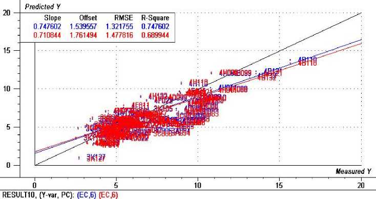
Figure 1. The prediction model using PLS as the regression model and full-cross-validation as the validation model.
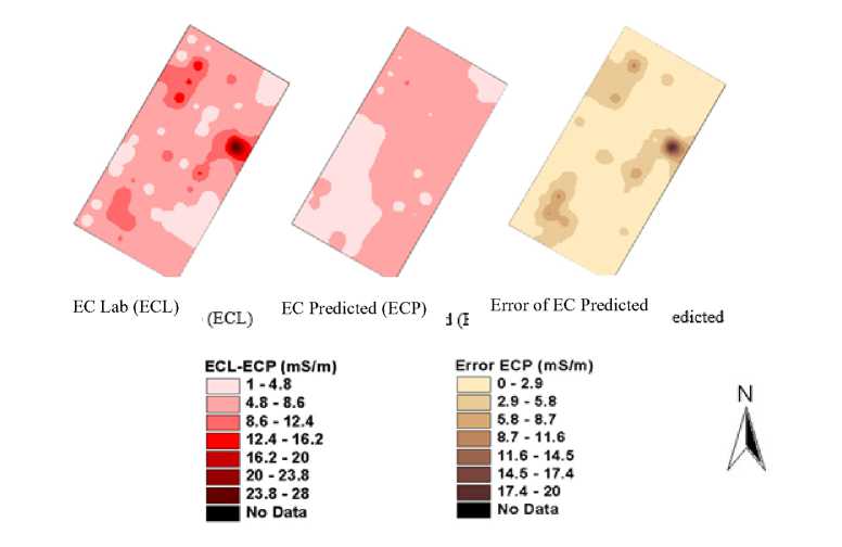
Figure 2. IDW Interpolation maps of soil EC in Field 3 generated from ECL (soil EC by lab analysis) ECP (predicted EC from spectra) and error map of ECP.
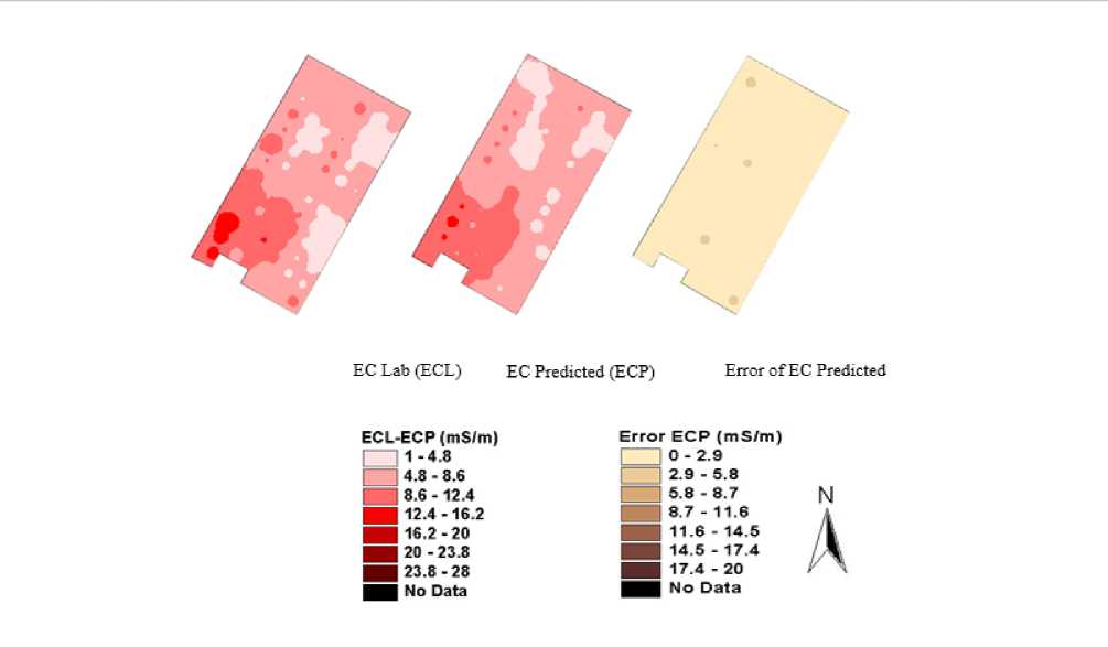
Figure 3. IDW Interpolation maps of soil EC in Field 4 generated from ECL (soil EC by lab analysis), ECP (predicted EC from spectra) and error map of ECP.
Figure 2 shows the spatial variability on soil EC between laboratory analyses (ECL) and spectra (ECP) with different method. Result showed that the EC records of ECP value were lower than ECL. The higher error comes from areas which have higher EC values. This means that the regression model has a limitation in predicting higher EC values (approximately 15 mS/m).
Figure 3 shows that field 3 has a similar spatial variability on ECL and ECP. The error of ECP is quite small as compared with the Error of ECP of Field 3. Error ECP is the difference between ECL
with ECP.
Capacitance method
Simple regression showed no correlation between ECL with soil EC front sensor (ECF) and side sensor (ECS) (
Figure 4 and Figure 5).
Figure 4 shows the correlation of ECL with EC front sensor and EC side sensor data records. EC data records was normalized using standard score normalization
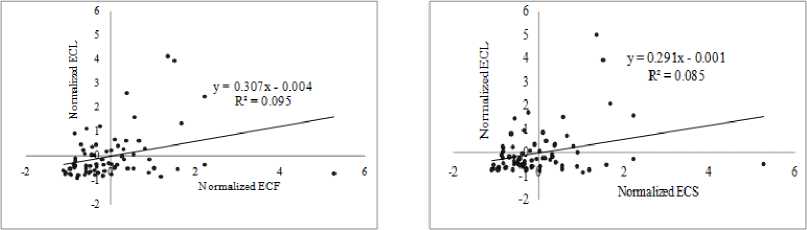
Figure 4. Correlation of soil EC by lab analysis records (ECL) with soil EC records at the front electrode of chisel tip (ECF) and soil EC records at the side electrode of chisel tip (ECS) field
3.
|
6 ⅛ 5 -j 4 3 3 I 2 |
y=0.48‰-0.000 R2 = 0240 |
|
-2 |
Normalized ECF |
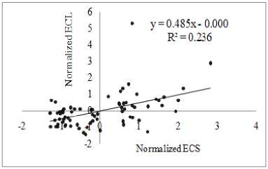
Figure 5. Correlation of soil EC by lab analysis records (ECL) with soil EC records at the front electrode of chisel tip (ECF) and soil EC records at the side electrode of chisel tip (ECS) field 4.
Using simple regression (Figure 6), the correlation of ECF and ECS shows positive correlation. This indicates front sensor and side sensor are capable to record soil EC data. The primary cause of the extreme differences between ECL, ECF and ECS values is likely related to the calibration of the capacitance sensor itself.
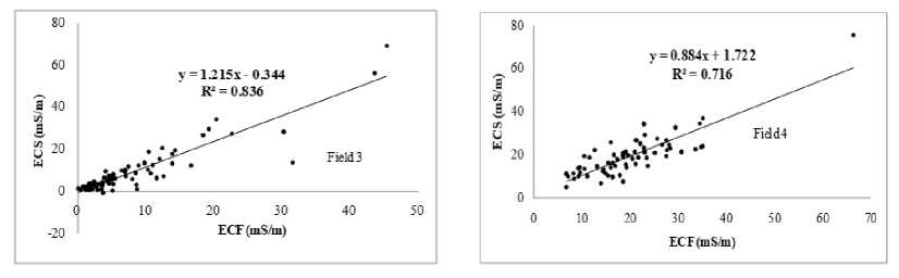
Figure 6. Correlation of soil EC records from at the front electrode of chisel tip (ECF) and Soil EC records at the side electrode of chisel tip (ECS).
Conclusions
Spectroscopic and capacitance methods are two approaches to measure bulk soil EC, but both approaches don’t appear to correlate well with each other. The spectroscopic method appears to have a positive correlation with soil EC laboratory analysis. In addition, capacitance methods need some adjustments so that both sensors may be utilized simultaneously and in a complementary fashion. By using a combined approach such as this, we should be able to maximize benefits from both methods while minimizing individual weaknesses.
A few variables may cause inaccuracies in capacitance sensor readings and need further investigation. Capacitance sensor re-calibration may be necessary to help correct for changes in these variables.
Fritz et al. 1999. Field comparison of two soil electrical conductivity measurement system. In: Roberth et al, proceeding of the fourth international conference on precision
agriculture. ASA-CSSA-SSSA. Michigan, p: 1211-1217
Shibusawa et al. 1999. Spectrophotometer for real-time underground soil sensing. An
ASAE Meeting Presentation Paper No. 993030. Toronto.
Sudduth et al, 2003. Comparison of electromagnetic induction and direct sensing of soil electrical conductivity. Agronomi Journal 95. 472-482.
References
Bulchleiter and Fahrani. 2002. Comparison of electrical conductivity measurement from two different sensing technologies. Paper No. 02-506, ASAE. Michigan.
13
Discussion and feedback