The Application Of Autoregressive Integrated Moving Average Generalized Autoregressive Conditional Heteroscedastic (Arima - Garch)
on
| 63
Udayana Journal of Social Sciences and Humanities, Vol. 4 No. 2, September 2020 DOI: https://doi.org/10.24843/UJoSSH.2020.v04.i02.p04
The Application Of Autoregressive Integrated Moving Average Generalized Autoregressive Conditional Heteroscedastic
(Arima - Garch)
(Case Study: Average National Retail Price for Rice in January 2007 - December 2017)
Pardomuan Robinson Sihombing. 1, Oki Prasetia Hendarsin 2 , Sarah Sholikhatun Risma3, Bekti Endar Susilowati4
* Corresponding author: BPS-Statistic Indonesia Email: robinson@bps.go.id, prasetiaoki@gmail.com, risma.sarah@bps.go.id, bekti@bps.go.id
Abstract Rice farming for Indonesia is vital. Rice farming is inseparable from the fact that rice farming is the livelihood of most of the population, while rice is the staple food of almost all Indonesians. The nature of rice that is easy to process and, following the public consumption culture, causes a very high dependence on rice. On the other hand, the price of rice is quite volatile. If the price of rice is soaring high, it can cause changes in the pattern of rice consumption. Some people want a stable supply and rice price, available at all times and evenly distributed and at affordable prices. Because the cost of rice is quite fluctuating, it is necessary to have a model that can be used to predict future rice prices so that the right policies can be implemented. Autoregressive Integrated Moving Average Model Generalized Autoregressive Conditional Heteroscedastic (ARIMA-GARCH) is a useful model for evaluating and predicting price fluctuations. This model's application is implemented in the national average retail rice price data between January 2007 and December 2017. In this study, rice data in the study period was not stationary at the level so that differentiating was carried out in the data. The best model is ARIMA (1,1,2) and Garch model (2,0). In this model, the data has complied with the white noise assumption, and the resulting GARCH model is free from the heteroscedasticity assumption.
Keywords: rice, volatility, ARIMA, GARCH.
Rice farming for Indonesia is essential. Rice farming is inseparable from the fact that rice farming is the livelihood of most of the population, while rice is the staple food of almost all Indonesians. The nature of rice that is easy to process and, following the culture of public consumption, causes a very high dependence on rice (Lastry, 2006). Prawiro (1998) argues that "... the Indonesian economy can be said to be a rice economy".
According to BPS data, Indonesia's per capita rice consumption per year averages 114.6 kg based on the 2017 National Socio-Economic Survey (SUSENAS) data collection. This amount is very far from other Asian countries such as Japan and Malaysia, which are only 60 kg and 80 kg per capita per year. The high consumption of rice in Indonesia shows how vital the rice commodity is for the Indonesian people.
Based on official government data, the average per capita rice consumption per week of the Indonesian population starting from 2007 was 1.74 million and reached 1.57 million in 2017. Rice production in 2007
was recorded at 57.15 million tonnes, then increased to 60.32 million tonnes in 2008. In 2009 it reached 64.39 million tonnes, and in 2010 it again increased to 66.47 million tonnes, likewise with the 2011-2017 period with an increasing trend of production, namely 65.75 million tons in 2011 and 81.38 million tons in 2017. Over the last ten years, there has always been an increase in national grain production.
Even though Indonesia's rice production is relatively high, this is also offset by increased consumption, which has led to the government's policy of importing rice. The government chose the import policy to meet domestic rice needs and reduce prices to keep it affordable for consumers. This is detrimental to farmers. Data collected from BPS shows that Indonesia imports an average of 0.94 million tons of rice per year. In 2007 Indonesia's rice imports reached 1.4 million tons, and until 2017 Indonesia still imported rice getting 0.3 million tons.
Household rice needs consist of the need for direct consumption and minimum supplies (Lastry, 2006). So
that the availability of rice needs to be appropriately maintained because the community is very sensitive to issues regarding rice, and this is closely related to prices (Lastry, 2006). For households with a steady income, an increase in rice prices will, of course, harm consumption patterns, thereby affecting the level of household welfare in general (Arifin, 1994).
If not balanced with a high increase in rice production, the high demand for rice will cause a shortage in the availability of rice in the market. If there is no effort to increase national rice production, there will be problems between the need for and the availability of rice with a widening gap. If the need to consume rice is higher, and rice availability is not followed, then the rice price in the market will increase. The soaring price of rice resulted in changes in rice consumption patterns. Some people want a stable supply and rice price, available at all times and evenly distributed and at affordable prices. Therefore, the availability of rice, both quality and quantity, must be adequately maintained.
Eliyawati (2014) states that data in the financial sector, such as price index, is usually random and has high volatility or heteroscedasticity. Volatility is a measure of the uncertainty of time series data, which is indicated by the fluctuation and time-series characterized by fluctuations and time series with non-homogeneous variations called time series data with conditional heteroscedasticity (conditional heteroscedasticity).
In 1982, Engle introduced the Autoregressive Conditional Heteroscedastic (ARCH) model to model heteroscedastic data. Bollerslev in 1986 introduced the Generalized Autoregressive Conditional Heteroscedastic (GARCH) model as an extension of the ARCH model. The GARCH model is a simpler model with fewer parameters than the high degree ARCH model.
ARCH and GARCH models are beneficial for evaluating and predicting price fluctuations. ARCH and GARCH models treat heteroscedasticity as a variant to be modeled so that the prediction results of the variability of errors can be known. These predictions are usually more interesting, especially in financial applications (Engle, 2001). These models can describe the characteristics of finance.
Several studies using the ARCH and GARCH methods in financial applications have been widely used, including: Analysis of the Volatility of Shares of Go Public Companies with the ARCH-GARCH method (Nastiti Suharsono, 2012), Application of the GARCH (Generalized Autoregressive Conditional Heteroscedasticity) Model to test the Capital Market Efficient in Indonesia (Eliyawati et al., 2014), Application of the GARCH Model to Indonesian Foodstuff Inflation Data (Santoso, 2011). In this research, the ARIMA method's theoretical analysis with the GARCH model is to estimate parameters and create a
model that will be applied to predict the average retail price of the national rice commodity.
Based on the description of the problem that has been formulated above, the objective to be achieved in this study is to determine the Autoregressive Integrated Moving Average Generalized Autoregressive Conditional Heteroscedastic (ARIMA-GARCH). This study also aims to apply the Autoregressive Integrated Moving Average Generalized Autoregressive Conditional Heteroscedastic (ARIMA-GARCH) model to the national average retail price data for the period of January 2007 - December 2017.
This study models the monthly data for the national average retail price of rice for the period January 2007-December 2017 using the ARIMA-GARCH model. An ARIMA-GARCH model was assessed, then followed by dignostic checking. Diagnostic checking is done to test the residuals which are white noise and heteroscedastic. The existence of heteroscedasticity is overcome by using the GARCH model. Data processing in this study uses software R 3.5.1.
The type of data used in this study is secondary data. Secondary data is data obtained from the UN non-profit organization World Food Program. The data source used comes from the monthly national average rice price data taken from January 2007 to December 2017, which is obtained from https://data.world/wfp/4fdcd4dc-5c2f-43af-a1e4-93c9b6539a27
Data Analysis
The steps for analyzing time data using the GARCH (p, q) model are as follows:
-
1. Perform the identification process by checking the observation data is stationary or not
-
2. Determine the model mean that fits by identifying the correlation structure captured by the model based on the ACF and PACF plots
-
3. Perform ARCH effect test (p) using the Lagrange Multiplier test
-
4. Then estimate the parameters of the GARCH model (p, q)
-
5. Perform a diagnostic check with the Ljung Box Pierce test
-
6. After obtaining a significant GARCH (p, q) model, select the best model by comparing the AIC and SIC values. The best model is the model that has the smallest AIC and SIC values
In this study, data on the average monthly retail price of national rice for January 2007-December 2017
were obtained from the UN non-profit organization World Food Program. The results of the descriptive analysis of the national average monthly retail rice price data are described in Table 1 below:
Table 1. Descriptive Statistics of National Retail
Average Rice Price
|
Minimum |
Maksi mum |
Rata-Rata |
Standar Deviasi |
|
5944 |
13676 |
9856 |
2618.281 |
Source: Author’s calculation
Based on Table 1, the national average retail price for rice is IDR 9,856. However, the national retail price for rice has reached the highest value, namely Rp. 13,676 occurred in December 2017, while the lowest price occurred in July 2007 at Rp. 5,944. When viewed from the amount of the data's standard deviation, the monthly average national retail rice price is relatively high, indicating fluctuation and forming an increasing trend.
-
3.2 Data Stationerity
A formal time-series data stationary check can be done using the Augmented Dickey-Fuller (ADF) test. The results of the ADF test using the R programming language are as follows:
Table 2. ADF Test Result
Dickey-Fuller = -2.0513, Lag order = 5, p-value = 0.5552
Source: Author’s calculation
With a significance level of 5%, from the test results shown in Table 2, it is found that H0 is not rejected (pvalue> 0.05), so it can be stated that the observed variables have not been stationary to the average, so it is necessary to do differencing. After differencing, time series data stationary checks were performed using the Augmented Dickey-Fuller (ADF) test. The results of the ADF test using the R programming language are as follows:
Table 1 ADF Test Result after Differencing
Augmented Dickey-Fuller Test
Dickey-Fuller = -4.7249, Lag order = 5, p-value = 0.01 Source: Author’s calculation
Based on Table 3 with a significance level of 5%, it is found that H0 is not rejected (p-value <0.05), so it can be stated that the observation variable has been stationary to the average. Thus, testing can proceed to the next stage.
ARIMA Effect Testing
In this process, the p value for AR (p) and the q value for MA (q) will be determined. For this purpose, select several ARIMA models, which will later be compared by the AIC values to get the best forecasting model. By using R programming, some of the ARIMA models that are formed are as follows:
Augmented Dickey-Fuller Test
Table 2 ARIMA Models
|
Model ARIMA |
AIC |
ar1 |
ar2 |
ma1 |
ma2 |
|
(2,1,2) |
1650.46 |
-0.6378794 |
0.9135411 |
2.043858* |
0.4781412 |
|
(2,1,1) |
1648.67 |
-0.5054924 |
0.8655849 |
6.348656* | |
|
(2,1,0) |
1650.3 |
7.208173* |
-3.053297* | ||
|
(1,1,2) |
1644.27 |
526.1424* |
-4.54014* |
-8.058272* | |
|
(1,1,1) |
1647.35 |
0.1111631* |
5.164483* | ||
|
(0,1,1) |
1645.36 |
9.252302* | |||
|
(0,1,2) |
1647.35 |
7.801257* |
0.0996632 |
Source: Author’s calculation
The ARIMA model (1,1,2) in Table 4 shows that the estimated parameters AR (1), MA (1), and MA (2) are statistically significant at α = 5%. Its AIC value is also the lowest compared to the other ARIMA models' estimation results, namely 1644.27. The estimation results in Table 4 are estimates of the ARIMA model without including ARCH / GARH elements. So, the detection whether the model contains heteroscedasticity problems or not is needed. If the model includes heteroscedasticity problems, then the ARMA model must be estimated using the ARCH / GARCH approach.
Steps that can be done is to detect the volatility of the error term. If the error term has high volatility, it indicates that the model contains heteroscedasticity problems.
GARCH Effect Testing
To prove that the ARIMA model used contains heteroscedasticity problems is to perform heteroscedasticity testing. In this paper, the PACF Residual Quadrat ARIMA (1,1,2) will be displayed.
DOI: https://doi.org/10.24843/UJoSSH.2020.v04.i02.p04
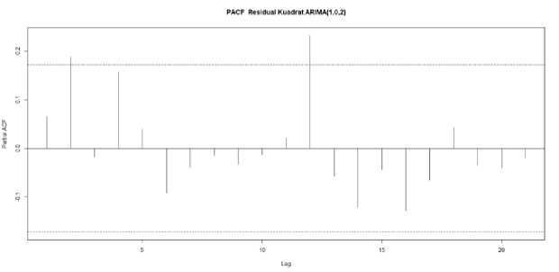
Figure 1 PACF Residual Squared ARIMA (1,1,2)
Based on Figure 1, the PACF plot of residual squared ARIMA (1,1,2), there is a second lag that comes out of the line, so it indicates a heteroscedasticity problem or contains GARCH elements. Apart from that, the plot also indicates that the best GARCH model is GARCH (2,0). Further exploration will be made for the GARCH model.
GARCH Estimation
Based on previous results, it is known that the ARIMA model (1,1,2) contains a heteroscedasticity effect so that it includes the GARCH element. The following table shows the estimation results after entering the two GARCH models:
Table 3 ARIMA-GARCH Modelling
|
Arima |
Garch |
mu |
ar1 |
ma1 |
ma2 |
|
(1,1,2) |
(2,0) |
2.00E+01* |
4.63E-01* |
-6.99E-03 |
-3.18E-01* |
|
(1,1,2) |
(1,0) |
1.69E+01* |
4.46E-01* |
-2.01E-01* |
-2.63E-01* |
|
Arima |
Garch |
omega |
alpha1 |
alpha2 |
AIC |
|
(1,1,2) |
(2,0) |
5.19E+03* |
1* |
2.15E-01 |
12.49784 |
|
(1,1,2) |
(1,0) |
6.22E+03P |
1* |
12.51961 |
Source: Author’s calculation
The output of the estimation results in Table 5, after entering the GARCH element, the results show a reasonably good estimation result. These results indicate that the national average monthly retail rice price data is significant by the error term's variant in the previous period, namely lags 1 and 2. The next step is to evaluate the estimation results in Table 5, whether they still
contain elements of heteroscedasticity or not. Tests are carried out using the LM test procedure. Based on the ARCH LM test shown in Table 6, it shows that the estimation results of the GARCH model in Table 5 are heteroscedasticity free, as evidenced by the LM Arch Test value, which has a p-value> 0.05.
Tabel 4. 4 Diagnostik Cek Model ARIMA GARCH
|
Arima |
Garch |
Jarque-Bera Test |
Shapiro-Wilk Test |
Ljung-Box Test |
LM Arch Test | |
|
(1,1,2) |
(2,0) |
4.40E-10 |
2.66E-06 |
0.839529 |
0.153918 | |
|
(1,1,2) |
(1,0) |
1.60E-08 |
1.34E-05 |
0.651068 |
0.15328 | |
Source: Author’s calculation
From the explanation above, the best model used is the ARIMA (1,1,2) -GARCH (2,0) model with the following equation:
Mean model: yt=0,2+0,46 yt-1 - 0,007 εt-1 -0,31 εt-2
Volatility model: σf2 = lσ2-1 + 0,2σt^2
From the coefficient and significance of the mean model, it can be interpreted that the increase in the price of rice in the previous period will increase the rice price in the next period, assuming other variables are constant. Likewise, the previous period's price volatility will increase the volatility of rice prices in the next period.
Based on the results of the study, it was found that the national average monthly rice retail price data
showed quite good behavior, even though it had relatively high volatility. As the stationarity test of the national retail rice monthly average price data is stationary to the average, so to analyze the volatility of the national retail rice monthly average price data, the approach of ARIMA, AR(p), d(1) dan MA (q) can be used. The ARIMA model's estimation results show that the best ARIMA models are AR (1), MA (2). However, after diagnosing heteroscedasticity, the ARIMA model that was selected contained heteroscedasticity elements. So, the GARCH method is used. The estimation results using the GARCH method show results that are not much different from the ARIMA method, but the main problems that are the focus of this study have been answered. The GARCH method can solve heteroscedasticity in time series data, which tends to high volatility due to the residual or error term containing heteroscedasticity elements. Regarding the case study, the increase in the price of rice in the previous period will increase the rice price in the next period, assuming other variables are constant.
With the completion of this research, I would like to thank Mr Dr.Toni Toharudin and my team who have helped a lot until the completion of all the outcomes in this research.
REFERENCES
-
[5] Engle, RF. 1982. Autoregressive Conditional Heteroscedasticity with Estimates of the Variance of United Kingdom Inflation. Journal of Econometrica, Vol. 4 No. 4:987-1007.
-
[6] Engle, RF. 2001. GARCH 101: The Use of ARCH/GARCH Models in Applied Econometrics. Journal of Econometrics Perspectives, 4:157-168.
-
[7] Lastry, Y enny. 2006. Analisis Pola Konsumsi Beras Rumah Tangga Di Kota Bogor. Skripsi Sarjana Sosial Ekonomi Pertanian, Fakultas Pertanian. Institut Pertanian Bogor.
-
[8] Nastiti, K. L. A. A. Suharsono. 2012. Analisis Volatilitas Saham Perusahaan Go Public dengan Metode ARCH-GARCH. Jurnal Sains dan Seni ITS, Vol. 1 No. 1.
-
[9] Prawiro, Radius. 1998. Pergulatan Indonesia membangun ekonomi : pragmatisme dalam aksi. Jakarta: Elex Media Komputindo.
-
[10] Santoso, T. 2011. Aplikasi Model GARCH pada Data Inflasi Bahan Makanan Indonesia. Jurnal Aset, Vol. 13 No. 1: 65-76.
-
[11] Tsay, R.S. 2005. Analysis of Financial Time Series. New York: A John Wiley Sonc, Inc. Publication, (Online)
-
[12] Wei, W. 2006. Time Series Analysis: Univariate and Multivariate Methods. NeJersey: Pearson Education, Inc.
-
[1] Arifin, Bustanul. 1994. Pangan dalam Orde Baru. Cetakan Kedua. Koperasi Jasa Informasi (Kopinfo). Jakarta
-
[2] Bollerslev. 1986. Generalized Autoregressive Conditional Heteroskedasticity. Journal of Econometrics, 31:307-327.
-
[3] Dianti, R.W. 2010. Kajian Karakteristik Fisikokimia dan Sensori Beras Organik Mentik Susu dan IR64, Pecah Kulit dan Giling Selama Penyimpanan.[Skripsi]. Universitas Sebelas Maret. Surakarta. Hal 5.
-
[4] Eliyawati, W. Y., R. R. Hidayat, D. F. Azizah. 2014. Penerapan Model GARCH (Generalized Autoregressive Conditional Heteroscedasticity) Untuk Menguji Pasar Modal Efisien Di Indonesia. Jurnal Administrasi Bisnis (JAB), Vol. 7 No. 2.
Discussion and feedback