Dissolved Oxygen Prediction of the Ciliwung River using Artificial Neural Networks, Support Vector Machine, and Streeter-Phelps

JURNAL ILMIAH MERPATI VOL. 10, NO. 3 DECEMBER 2022            p-ISSN: 2252-3006

e-ISSN: 2685-2411

Dissolved Oxygen Prediction of the Ciliwung River using Artificial Neural Networks, Support Vector Machine, and Streeter-Phelps

Yonas Prima Arga Rumbyarso^a1, Nuke L. Chusna^b2, Ali Khumaidi^b3

^aCivil Department, Faculty of Engineering, Universitas Krisnadwipayana, Indonesia ^bInformatic Department, Faculty of Engineering, Universitas Krisnadwipayana, Indonesia e-mail: ¹[email protected], ²[email protected], ³[email protected]

Abstrak

Evaluasi kualitas air sungai Ciliwung dapat dilakukan dengan menganalisis distribusi dissolved oxygen (DO). Tujuan dari penelitian ini adalah untuk menganalisis parameter lingkungan yang berpengaruh terhadap sebaran DO, dengan melakukan pemodelan prediksi untuk menduga sebaran DO di Sungai Ciliwung. Data penelitian menggunakan data primer dan data sekunder yang sebagian data diperoleh dari penelitian sebelumnya. Parameter kualitas air yang digunakan yaitu DO, suhu, biochemical oxygen demand (BOD), chemical oxygen demand (COD), power of hydrogen (pH) dan kekeruhan. Dataset yang digunakan terdapat missing value sebesar 28.8%, untuk optimalisasi hasil model dilakukan praprocessing menggunakan pendekatan machine learning yaitu membandingkan algoritme support vector machine (SVM), artificial neural network (ANN) dan linier regression. Tiga model dibandingkan untuk memprediksi DO, hasil evaluasi kinerja model SVM, ANN dan Streeter-Phelps memiliki nilai RMSE sebesar 0.110, 0.771, dan 0.114. SVM memiliki kinerja terbaik dalam memprediksi DO.

Kata kunci: ANN, Kualitas Air, Oksigen Terlarut, Streeter-Phelps, SVM

Abstract

Evaluation of Ciliwung river water quality can be done by analyzing the distribution of dissolved oxygen (DO). The purpose of this research is to analyze the environmental parameters that affect the distribution of DO, by carrying out predictive modeling to estimate the distribution of DO in the Ciliwung River. The research data used primary data and secondary data, some of which were obtained from previous studies. The water quality parameters used are DO, temperature, biochemical oxygen demand, chemical oxygen demand, power of hydrogen, and turbidity. The dataset used has a missing value of 28.8%. To optimize the model results, preprocessing is carried out using a machine learning approach, namely comparing support vector machine (SVM), artificial neural networks (ANN), and linear regression. The three models were compared to predict DO, the results of performance evaluation of the SVM, ANN and Streeter-Phelps models had RMSE values of 0.110, 0.771, and 0.114.

Keywords : ANN, Dissolved Oxygen, Streeter-Phelps, SVM, Water quality

stipulated in the quality standard. The Ciliwung River Basin (DAS) has a strategic function in a national context, so it needs to be managed specifically. The length of the Ciliwung river from upstream to downstream in Jakarta Bay is ± 117 km with a catchment area of 347 km2. The Ciliwung watershed covers the upstream area in the Puncak area, Bogor Regency, to the downstream area in Jakarta Bay [6]. The damage that occurred to the Ciliwung river was caused by human activities in the vicinity of the Ciliwung watershed. Various policies that did not pay attention to environmental aspects were allegedly one of the factors causing the destruction of the Ciliwung watershed. This is then exacerbated by the presence of industrial waste in the middle segment of the Ciliwung watershed and the presence of domestic waste from people who live along the Ciliwung River which further degrades the quality of Ciliwung river water [7].

Efforts that can be made in evaluating the quality of Ciliwung river water is to analyze the distribution of dissolved oxygen or dissolve oxygen (DO) in the Ciliwung river. Oxygen (O2) is essential for life and a critical constraint on aquatic ecosystems [8][9]. DO is one of the important parameters in determining water quality because it can indicate the level of pollution in a water. DO concentration in waters reflects the equilibrium of oxygen production and oxygen consumption processes. This process is highly dependent on various factors such as temperature, salinity, oxygen depletion, oxygen source and other water quality parameters [10]. Water quality is influenced by various factors which in fact have quite complicated non-linear relationships with various variables such as traditional data processing methods which are no longer feasible to solve the problem. Several things such as speed, accuracy, time efficiency and cost are also some of the factors that can influence river water quality monitoring. Thus it is necessary to have the latest innovations in monitoring water quality in the form of using artificial intelligence in monitoring water quality [11]. The purpose of this research is to analyze the environmental parameters that influence the distribution of dissolved oxygen, to conduct prediction modeling to predict the distribution of dissolved oxygen in the Ciliwung River using an artificial neural network (ANN) and a support vector machine (SVM), and to analyze the differences in the results of modeling the distribution of dissolved oxygen. between ANN, SVM and the Streeter-Phelps model. The results of this study can provide information regarding the quality of river water as a source of water used in daily activities.

• 2.    Research Method and Materials

The stages of this research are presented simply in the form of a flowchart in Figure 1. This research uses the Ciliwung River water quality dataset for modeling dissolved oxygen using ANN. The variables used are variables affecting the value of dissolved oxygen in river water, in the form of power of hydrogen (pH), temperature, turbidity, chemical oxygen demand (COD) and biochemical oxygen demand (BOD). The dataset used is a primary dataset obtained from research by Astono [12], Hendrawan [13], Rahman [14], Soewandita [7], and secondary data obtained by researchers. The data used is 55, the sample dataset can be seen in Table 1.

Figure 1. Research stages

The dataset that will be used as ANN and SVM learning data consists of six parameters which are divided into input and output data. In building the model, it is necessary to analyze the correlation between parameters. The purpose of the correlation analysis is to find out whether the relationship between these parameters is positive or negative. Before modeling the preprocessing stage is carried out to overcome the presence of missing values in the dataset. Missing value in the dataset is 28.8%. The approach used is machine learning, which uses the SVM, ANN and linear regression algorithm. For DO prediction modeling compare ANN, SVM and Streeter-Phelps. Calculations in the Streeter-Phelps modeling are the deoxygenation constant and the re-aeration constant. Calculations on both constants are carried out with empirical formulas related to hydraulic parameters, namely velocity and depth of flow. Model performance is assessed based on the value of the coefficient of determination (R2) and the root mean square error (RMSE) value.

Table 1. Dataset samples
No	DO	PH	Temperature	Turbidity	BOD	COD
1	3,38	7,57	19,2	62,91	3,83	5,77
2	4,35	7,9	22	50,89	4,6	12
3	3,23	7,88	25,4	64,77	5,9	16
4	0,02	7,47	26,8	104,55	11,1	17,31
5	0,01	7,17	27,6	104,67	12,2	28,35
6	0,89	7,15	27	93,76	10,1	20
7	0,82	7,15	27,6	94,63	6,45	36,54
8	0,82	7,15	27,5	94,63	11,85	40,38
9	0,86	6,8	28	94,14	11,1	40,38
10	0,76	6,9	28	95,38	30,18	36,54
11	3,5	7,1	27,9	?	15	27
12	3,3	7,4	29,1	?	25	25
13	3,5	6,9	29,2	?	14	28
14	3,5	6,9	29,6	?	12	23
15	3,2	7,1	30,4	?	27	57
... 53	... 5,64	... 6,04	... 27,6	... 37,1	... ?	... ?
54	5,54	6,04	27,5	37,3	?	?
55	5,44	6,04	27,7	37,5	?	?

• 3.    Literature Study
  
  3.1.    Water quality

Water quality is a term to describe the condition of water that will be used for its designation such as drinking water, fisheries, irrigation, industry, and so on [15]. Water quality includes three characteristics, namely physics, chemistry and biology. Several water quality parameters include pH, color, electrical conductivity temperature, chemical substance concentration, bacterial concentration, and so on. The following are some of the parameters that affect water quality: a. Dissolved Oxygen

Dissolved Oxygen (DO) is the amount of oxygen dissolved in a water. DO is needed by all microorganisms in the waters to be used in respiration processes, metabolism so that microorganisms can produce energy for growth and reproduction [16]. The amount of oxygen needed by microorganisms is highly dependent on the amount of water and the type of organic matter contained in the waters. Therefore, the entry of organic waste from household, industrial, mining and agricultural activities will reduce O2 levels in water [17]. Thus, the higher the DO value contained in a water, the better the water quality.

• b.    Power of Hydrogen

Power of Hydrogen (pH) or degree of acidity is the intensity of acidity or alkalinity of a liquid and represents the concentration of hydrogen ions in a solution. The degree of acidity is an important parameter in analyzing water quality. This is because pH has a significant influence on the biological and chemical processes in it [18]. Water that comes from the mountains usually has a high pH. The pH value of this water will decrease as the water flows from the mountains to the downstream. This is due to the addition of organic matter which is able to release CO2 so that the pH of the water will decrease. The pH value greatly affects the physical, chemical and biological processes of organisms that live in waters. The pH value greatly influences the toxicity of polluting materials and the solubility of some gases, and determines the form of substances in water [19].

• c.    Biochemical Oxygen Demand

Biochemical Oxygen Demand (BOD) is the amount of dissolved oxygen needed by microorganisms living in the aquatic environment to decompose or degrade organic waste substances contained in the aquatic environment. BOD serves to measure the amount of oxygen used by microbial populations in waters in response to the entry of organic matter that can be decomposed [20]. The BOD value is expressed in milligrams of oxygen per liter.

• d.    Chemical OxygenDemand

Chemical Oxygen Demand (COD) is the amount of oxygen needed to decompose all organic matter contained in water and the COD value can be obtained by the oxygen value needed to decompose all organic matter in waters. This is because in the process of determining the value of COD, the chemical potassium bichromate is used in acidic and hot conditions with a silver sulfate catalyst so that organic matter that is easily decomposed or that is difficult to decompose will be oxidized [21].

• e.    Temperature

Temperature is a measure or degree of hotness or coldness of a system or object [22]. Temperature is one of the factors that can affect chemical reactions and biological activity in waters. Temperature plays a very important role in controlling the condition of aquatic ecosystems, especially on the survival of an organism. An increase in temperature in water bodies can result in a decrease in the amount of dissolved oxygen in the water, an increase in the speed of chemical reactions and the life of fish and other aquatic animals becomes disrupted [23]. Increasing temperature also causes an increase in the decomposition of organic matter by microbes. In addition, river water temperature is a limiting factor for aquatic organisms [24]. Thus, changes in surface temperature can affect the physical, chemical and biological processes that occur in these waters [25].

• f.    Turbidity

Turbidity is the amount of granular substance contained in water that cannot be seen by the naked eye. Turbidity in water is not part of the water's harmful properties. However, turbidity can cause fear of the presence of chemical compounds in water that can endanger life. The level of water turbidity is commonly referred to as turbidity. Turbidity in waters is generally caused by the presence of suspended particles such as clay, silt, dissolved organic materials, bacteria, plankton and other organisms. This turbidity level is usually referred to as nephelometric turbidity units (NTU). According to WHO (1998), the level of turbidity in drinking water has a maximum limit that meets the requirements of 5 NTU.

• 3.2.    ANN and SVM modeling

Artificial Neural Network (ANN) is an information processing system inspired by biological neural networks in the human body so that Artificial Neural Networks have characteristics similar to biological neural networks in humans [26]. ANN is also known as a general form of mathematical modeling in human biological neural networks [27]. ANN is often used in the development of predictive models. This is because ANN can model quite complex problems which are very difficult to model in the form of mathematical equations [28]. ANN has the ability to recognize and study the relationship between system inputs and outputs without paying attention to their physical form explicitly [29]. The ANN architecture can be seen in Figure 2.

Modeling a problem by ANN can be done with the backpropagation method. The ANN backpropagation method is an ANN technique using a forward and backward learning system that is based on an error backpropagation algorithm with error correction[30]. This network consists of various layers. The input layer will be connected to the hidden layer. The hidden layer will be connected to the output layer. When given an input pattern, the pattern will go to the hidden layer and be forwarded to the output layer. If the output results are not as expected, then the output will be propagated backwards to the hidden layer and then to the input layer [31].

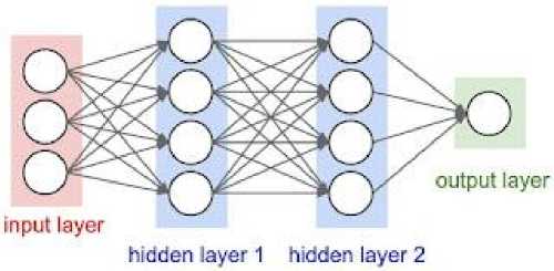
Figure 2. Architecture of the Multi Layer ANN Model

Support Vector Machine (SVM) is a method in supervised learning which is usually used for classification (Support Vector Classification) and regression (Support Vector Regression (SVR)). The SVR algorithm is a theory adapted from machine learning theory that has been used to solve classification problems, namely SVM. This SVR is the application of the SVM algorithm in the regression case. In the SVM method is the application of machine learning theory to classification cases that produce integer values, while the SVR algorithm is the application of regression cases which produce output in the form of real numbers [32]. The concept of the SVR algorithm can produce good forecasting values because SVR has the ability to solve overfitting problems. Overfitting is data behavior during the training or training phase resulting in almost perfect prediction accuracy. The goal of the SVR algorithm is to find a dividing line or it can be called the best hyperplane. The best hyperplane can be found by measuring magin with that hyperplane. Margin itself is the distance from the hyperplane to the closest data. The closest data from the margin is called the support vector[33].

• 3.3.    Streeter-Phelps modeling

The Streeter-Phelps model is a model for determining the carrying capacity of water pollution loads by applying a mathematical calculation approach to the mass balance of a water by assuming one dimension and in steady state. Streeter-Phelps modeling uses the oxygen sag curve equation [34]. Streeter-Phelps modeling is generally limited to discussing only two phenomena, namely:

• a.    The process of reducing dissolved oxygen (deoxygenation) due to bacterial activity in degrading organic matter in water.

• b.    The process of increasing dissolved oxygen (reaeration) caused by turbulence that occurs in river flow.

• 3.4.    Performance evaluation

Model performance is assessed based on the value of the coefficient of determination (R²) and the root mean square error (RMSE) value. The value of R² > 0.7 indicates that a model is very good, whereas if the value of R² <0.4 then the prediction model should not be used.

• 4.2.    Data Preprocessing

In the dataset, it can be seen that the parameters experiencing missing values are temperature, turbidity, BOD, and COD. To overcome missing values, machine learning techniques are carried out using the SVM, ANN and linear regression (LR) algorithms. The three algorithms were compared and the algorithm with the best performance was selected for the prediction of missing values in the parameters. For prediction of temperature parameters the best algorithm is LR with R² of 0.645, for prediction of turbidity and BOD parameters using the best algorithm is SVM and for prediction of COD parameters the best algorithm is ANN. Table 2 presents the results of the comparison of the three algorithms in parameter prediction and the results of filling in the missing values with the selected algorithm for each parameter can be seen in Table 3.

Table 2. Result of algorithm comparison results for parameter prediction

	Tempe	tature	Turbidity	BOD	R2	COD
	RMSE	R2	RMSE    R2	RMSE		RMSE    R2
SVM	1,464	0,607	5,691    0,953	13,606	-0,103	19,353    0,306
ANN	16,533	-5,687	12,642    0,767	15,368	0,407	18,87    0,341
LR	1,39	0,645	5,775    0,951	15,055	0,351	18,984    0,333
		Table 3.	Dataset samples	after preproce	ssing
No	DO	PH	Temperature	Turbidity	BOD	COD
1	3,38	7,57	19,2	62,91	3,83	5,77
2	4,35	7,9	22	50,89	4,6	12
3	3,23	7,88	25,4	64,77	5,9	16
4	0,02	7,47	26,8	104,55	11,1	17,31
5	0,01	7,17	27,6	104,67	12,2	28,35
6	0,89	7,15	27	93,76	10,1	20
7	0,82	7,15	27,6	94,63	6,45	36,54
8	0,82	7,15	27,5	94,63	11,85	40,38
9	0,86	6,8	28	94,14	11,1	40,38
10	0,76	6,9	28	95,38	30,18	36,54
11	3,5	7,1	27,9	73,39	15	27
12	3,3	7,4	29,1	74,6	25	25
13	3,5	6,9	29,2	76,07	14	28
14	3,5	6,9	29,6	79,33	12	23
15	3,2	7,1	30,4	69,84	27	57
... 53	... 5,64	... 6,04	... 27,6	... 37,1	... 34,8	... 44,51
54	5,54	6,04	27,5	37,3	34,89	44,64
55	5,44	6,04	27,7	37,5	34,97	44,78

• 4.3.    ANN and SVM modeling

In building prediction models using ANN and SVM algorithms. In ANN modeling using a model consisting of 3 layers, namely input, hidden layer, and output. In the hidden layer compared to the use of 1 hidden layer with 100 neurons and 2 hidden layers with 100 neurons each. To activate it, use Relu and the solver is Adam. Whereas SVM uses a linear kernel and both with 1000 iterations. The splitting of training data and testing data is 80 and 20. The results of the comparison of ANN and SVM can be seen in Table 4. The results of the prediction of dissolved oxygen using SVM and ANN modeling show that SVM outperforms ANN with 2 hidden layers and 1 hidden layer. SVM has an RMSE of 0.101 and an R2 of 0.998.

Table 4. Results of SVM and ANN modelling RMSE       R²

SVM	0,101	0,998
ANN (1 hidden layer)	0,694	0,928
ANN (2 hidden layer)	0,510	0,961

• 4.4.    Comparison of ANN, SVM and streeter-phelps modeling

The most frequently used water quality modeling method is the Streeter-Phelps modeling method. Streeter-Phelps modeling is carried out using various test model equations which have differences in each test model. Analytical calculations using the Streeter-Phelps model are carried out based on hydraulic factors that affect dissolved oxygen levels. Several hydraulic parameters that can affect dissolved oxygen levels are distance, depth, and speed at each point/segment.

Streeter-Phelps modeling is done by performing a series of calculations related to the deoxygenation constant and the re-aeration constant. The two constants are calculated using river hydraulics parameters. The deoxygenation constant is calculated using an empirical formula that takes into account situational factors in the field such as river depth. The depth of the river greatly affects the level of dissolved oxygen. The deeper the river, the less concentration there is so that the fewer microorganisms that live in the river. The ability to rearate can increase dissolved oxygen levels in water because oxygen from the atmosphere diffuses with water. A large value of the reaeration constant will result in more oxygen diffusing into the river, resulting in high dissolved oxygen levels and reducing the potential for oxygen deficit.

The results of the calculation of the deoxygenization constant and the reaeration constant are then used in constructing a dissolved oxygen model using the Streeter-Phelps modeling method. The Streeter-Phelps mathematical model equation used is listed in Table 5. After the model is formed, then an analysis of the accuracy of the model is carried out. In testing the comparison of the ANN, SVM and Streeter-Phelps models, 10 datasets were used. The results of the Streeter-Phelps modeling of all equations can be seen in Table 6. The level of accuracy of the model was carried out using several statistical tests, namely the coefficient of determination, the bias factor and the RMSE value. The test value of the Streeter-Phelps model statistical analysis is presented in Table 7. It can be seen that the best model uses the 9th equation, namely BI with an RMSE value of 0.114. And the results of the comparison of the three DO prediction models can be seen in Table 8. From the 10 datasets tested using 3 dissolved oxygen prediction models, the Streeter-Phelps RMSE value is 0.114, the RMSE from SVM is 0.110, and the RMSE from ANN is 0.771.

Table 5. Reaeration constant equation
Number of Equation	Research Related	Abbreviation	Equation
1	Owens et al. (1964 )	OW	k2=〖5.32v〗^0.67/H^1.85
2	Langbein dan Darum (1967)	LD	k2=5.134v/H^1.33
3	Churcill et al. (1962)	CH	k2=5.026v/H^1.67
4	O'Connor dan Dobins (1958)	OD	k2=〖3.93v〗^0.5/H^1.5
5	Issacs et al. (1969)	IS	k2=4.05v/H^1.5
6	Negulescu dan Rojanski (1969)	NR	k2=〖10.9v〗^0.85/H^0.85
7	Bansal (1973)	BA	k2=〖4.1528v〗^0.6/H^1.4
8	Bennet dan Rathburn (1972)	BR	k2=〖5.5773v〗^0.607/H^1.689
9	Baecheler dan Lazo (1999)	BL	k2=〖1.923v〗^1.325/H^1.689
10	Jha et al. (2001)	JH	k2=〖5.729v〗^0.5/H^0.25
11	Padden dan Gloyna (1972)	PG	k2=〖10.9v〗^0.85/H^0.85

12	Eloubaldy (1969)	EL	k2=10.9v/H^1.5
13	Susanto et al. (2016)	SU	k2=〖5.144v〗^0.251/〖(0.5H)〗^(-0.3
14	Omole dan Longe (2012)	OL	k2=〖46.2679v〗^1.5463/H^0.0128
15	Agunwamba et al. (2007)	AG	k2=〖11.6325v〗^1.0954/H^00016
16	Issacs dan Gaudy (1968)	IG	k2=4.7531v/H^1.5
17	Ling et al. (2010)	LI	k2=〖1.923v〗^0.273/(2.303H^1.33
18	Boulton (1954)	BO	k2=5.32v/H^1.67
19	NIH (2000)	NI	k2=〖6.244v〗^0.558/H^0.234

Information:

V	: Average speed (m.second)
H	: Average depth (m)
K2	: Reaeration constant (day-1)
T	: Sample temperature (c)

		Table 6.	Result of Streeter-Phelps modeling
Testing data	OW	LD	CH	OD	IS	NR	BA	BR	BL	JH
(Actual)	(1)	(2)	(3)	(4)	(5)	(6)	(7)	(8)	(9)	(10)
3,38	3,38	3,38	3,38	3,38	3,38	3,38	3,38	3,38	3,38	3,38
4,35	8,51	8,23	8,35	8,43	8,14	8,47	8,38	8,51	7,00	8,20
3,23	3,03	3,12	2,75	3,40	2,73	5,65	3,43	3,39	2,06	6,71
0,002	4,27	4,12	3,18	4,74	2,83	7,33	4,78	5,08	-0,92	7,48
0,001	2,71	2,28	1,50	3,32	1,22	6,41	3,26	3,56	-1,34	6,93
0,89	1,54	1,57	1,32	1,64	1,24	3,65	1,68	1,78	0,63	3,89
0,82	1,16	1,06	0,90	1,31	0,85	2,67	1,30	1,38	0,44	3,22
0,82	1,22	1,19	1,12	1,20	1,06	2,05	1,21	1,31	0,80	1,88
0,86	2,35	1,46	1,19	2,73	0,97	4,52	2,50	2,92	-0,26	5,25
0,76	1,50	1,00	0,85	1,72	0,74	2,96	1,59	1,84	0,12	3,57
Testing data	PG	EL	SU	OL	AG	IG	LI	BO	NI
(Actual)	(11)	(12)	(13)	(14)	(15)	(16)	(17)	(18)	(19)
3,38	3,38	3,38	3,38	3,38	3,38	3,38	3,38	3,38	3,38
4,35	8,47	8,14	8,19	8,48	8,05	8,25	1,76	8,36	8,20
3,23	5,65	2,73	7,87	7,78	6,97	2,86	2,01	2,78	6,74
0,002	7,33	2,83	7,75	7,80	7,60	3,41	-2,17	3,33	7,50
0,001	6,41	1,22	7,57	7,55	7,00	1,68	-1,91	1,61	6,94
0,89	3,65	1,24	5,81	7,07	4,77	1,38	0,43	1,36	3,97
0,82	2,67	0,85	5,40	5,24	3,32	0,94	0,37	0,93	3,24
0,82	2,05	1,06	2,56	4,54	2,37	1,11	0,69	1,14	1,92
0,86	4,52	0,97	7,00	5,94	4,40	1,21	-0,42	!   1,26	5,18
0,76	2,96	0,74	5,73	4,26	2,86	0,86	0,05	0,89	3,51
	Table 7	Results of Statistical Analysis of the Streeter-Phelps Model
Model	CorrelationCoefficient (R)			R2		BF	RMSE		Peringkat
BL		0,942		0,887		-		0,114		1
LI		0,863		0,744		-		0,852		2
IS		0,812		0,659		4,779		1,027		3
EL		0,812		0,659		5,289		1,027		4
CH		0,786		0,617		5) 65		1,089		5

BO	0,736	0,542	5,833	0,996	6
IG	0,733	0,537	5,852	1,113	7
LD	0,722	0,522	5,549	1,208	8
OW	0,689	0,475	6,619	1,294	9
OD	0,638	0,406	7,250	1,372	10
BA	0,648	0,419	7,081	1,360	11
BR	0,607	0,369	7,528	1,416	12
PG	0,320	0,102	11,357	1,826	13
NR	0,320	0,102	11,357	1,826	14
JH	0,272	0,074	12,257	1,913	15
AG	0,232	0,054	13,141	1,919	16
NI	0,234	0,055	13,006	1,915	17
OL	0,087	0,008	16,653	2,184	18
SU	0,066	0,004	16,134	2,165	19

Table 8. Results of comparison of prediction models

Testing data (Actual)	SVM	Predict ANN	Streeter-Phelps
3,38	3,48	5,66	3,38
4,35	4,5	4,88	7,00
3,23	3,35	3,69	2,06
0,002	0,09	0,32	-0,92
0,001	0,09	0,04	-1,34
0,89	0,9	0,84	0,63
0,82	0,93	0,7	0,44
0,82	0,98	0,55	0,80
0,86	0,94	1,09	-0,26
0,76	0,9	0,61	0,12

• 5. Conclusion

After analyzing the relationship between water quality and dissolved oxygen, prediction models to estimate DO distribution in the Ciliwung River were compared, namely SVM, ANN, and Streeter-Phelps. The machine learning approach was chosen to overcome the missing value of 28.8%. After preprocessing the SVM and ANN modeling datasets, both of them produced quite good performance with R2 of 0.998 and 0.961. Streeter-Phelps modeling has various empirical equations in predicting DO, the use of the model developed by Baechelor and Lazo has an R2 value of 0.887. The results of the comparison of the three models show that SVM has the most superior performance compared to ANN and Streeter-Phelps, with an RMSE of 0.110. Previous research stated that ANN has better performance compared to Streeter-Phelps [14].

Acknowledgments

The authors would like to thank the Ministry of Education, Culture, Research and Technology (Kemdikbudristek) of the Republic of Indonesia for funding research in 2022.

References

• [1]    J. Afrianto L, Rohmat D, “Proyeksi kebutuhan air bersih penduduk Kecamatan

Indramayu Kabupaten Indramayu sampai tahun 2035,” Antol. Geogr., vol. 2, no. 3, pp. 1–12, 2018.

• [2]    S. O. Ningrum, “Analysis Quality of Water River and Quality of Well Water in The

Surrounding of Rejo Agung Baru Sugar Factory Madiun,” J. Kesehat. Lingkung., vol. 10, no. 1, p. 1, Aug. 2018, doi: 10.20473/jkl.v10i1.2018.1-12.

• [3]    Pengelolaan Kualitas Air dan Pengendalian Pencemaran Air. Pemerintah Republik

Indonesia, 2001.

• [4]    D. H. Kumar Reddy and S. M. Lee, “Water Pollution and Treatment Technologies,” J.

Environ. Anal. Toxicol., vol. 02, no. 05, 2012, doi: 10.4172/2161-0525.1000e103.

• [5]    E. Yogafanny, “Pengaruh Aktifitas Warga di Sempadan Sungai terhadap Kualitas Air

Sungai Winongo,” J. Sains &Teknologi Lingkung., vol. 7, no. 1, pp. 29–40, Apr. 2015, doi: 10.20885/jstl.vol7.iss1.art3.

• [6]    S. Yudo and N. I. Said, “Status Kualitas Air Sungai Ciliwung di Wilayah DKI Jakarta

Studi Kasus: Pemasangan Stasiun Online Monitoring Kualitas Air di Segmen Kelapa Dua – Masjid Istiqlal,” J. Teknol. Lingkung., vol. 19, no. 1, p. 13, Mar. 2018, doi: 10.29122/jtl.v19i1.2243.

• [7]    H. Soewandita and N. Sudiana, “Studi Dinamika Kualitas Air Das Ciliwung,” J. Air

Indones., vol. 6, no. 1, Feb. 2018, doi: 10.29122/jai.v6i1.2449.

• [8]     D. Breitburg et al., “Declining oxygen in the global ocean and coastal waters,” Science

(80-. )., vol. 359, no. 6371, Jan. 2018, doi: 10.1126/science.aam7240.

• [9]    R. J. Diaz and R. Rosenberg, “Spreading Dead Zones and Consequences for Marine

Ecosystems,” Science (80-. )., vol. 321, no. 5891, pp. 926–929, Aug. 2008, doi:

10.1126/science.1156401.

• [10]    K. Edwin Kimutai, K. Emmanuel Chessum, and K. Job Rotich, “Dissolved oxygen modelling using artificial neural network: a case of River Nzoia, Lake Victoria basin, Kenya,” J. Water Secur., vol. 2, no. 1, Nov. 2016, doi: 10.15544/jws.2016.004.

• [11]   Yudha, “Aplikasi jaringan syaraf tiruan untuk memprediksi kualitas air sungai di Titik

Jembatan Jrebeng Kabupaten Gresik,” Universitas Brawijaya, 2017.

• [12]   W. Astono, M. S. Saeni, B. W. Lay, and S. Soemarto, "The DO-BOD Model

Develompent for Ciliwung River Water Quality Managemen," Forum Pascasarjana, Vol. 31, No. 1 Januari 2008:37-45

• [13]    D. Hendrawan, "Water Quality of Ciliwung River Refer to Oil and Grease Parameter," Jurnal Ilmu-ilmu Perairan dan Perikanan Indonesia, Desember 2008, Jilid 15, Nomor 2: 85-93

• [14]    I. F. Rahman and C. Arif, "Aplikasi Jaringan Syaraf Tiruan (JST) dalam Analisis Sebaran Oksigen Terlarut di Sungai Ciliwung,", Thesis, Civil and Environmental Engineering, IPB University

• [15]    J. C. Egbueri, P. D. Ameh, and C. O. Unigwe, “Integrating entropy-weighted water quality index and multiple pollution indices towards a better understanding of drinking water quality in Ojoto area, SE Nigeria,” Sci. African, vol. 10, p. e00644, Nov. 2020, doi: 10.1016/j.sciaf.2020.e00644.

• [16]    F. Salmasi, J. Abraham, and A. Salmasi, “Effect of stepped spillways on increasing dissolved oxygen in water, an experimental study,” J. Environ. Manage., vol. 299, p. 113600, Dec. 2021, doi: 10.1016/j.jenvman.2021.113600.

• [17]    M. G. Hutchins, G. Harding, H. P. Jarvie, T. J. Marsh, M. J. Bowes, and M. Loewenthal, “Intense summer floods may induce prolonged increases in benthic respiration rates of more than one year leading to low river dissolved oxygen,” J. Hydrol. X, vol. 8, p. 100056, Aug. 2020, doi: 10.1016/j.hydroa.2020.100056.

• [18]    R. Ueki, Y. Imaizumi, Y. Iwamoto, H. Sakugawa, and K. Takeda, “Factors controlling the degradation of hydrogen peroxide in river water, and the role of riverbed sand,” Sci. Total Environ., vol. 716, p. 136971, May 2020, doi: 10.1016/j.scitotenv.2020.136971.

• [19]    G. Zhu et al., “Impact of landscape dams on river water cycle in urban and peri-urban areas in the Shiyang River Basin: Evidence obtained from hydrogen and oxygen isotopes,” J. Hydrol., vol. 602, p. 126779, Nov. 2021, doi: 10.1016/j.jhydrol.2021.126779.

• [20]    H. Lv, Q. Yang, Y. Chen, X. Xu, C. Liu, and J. Jia, “Determination of seawater biochemical oxygen demand based on in situ cultured biofilm reactor,” J. Electroanal. Chem., vol. 903, p. 115872, Dec. 2021, doi: 10.1016/j.jelechem.2021.115872.

• [21]    A. A. M. Ahmed, “Prediction of dissolved oxygen in Surma River by biochemical oxygen demand and chemical oxygen demand using the artificial neural networks (ANNs),” J. King Saud Univ. - Eng. Sci., vol.  29, no. 2, pp.  151–158, Apr.  2017, doi:

10.1016/j.jksues.2014.05.001.

• [22]   B. S. Supu I, Usman B, “Pengaruh suhu terhadap perpindahan panas pada material

yang berbeda,” J. Din., vol. 7, no. 1, pp. 62–73, 2016.

• [23]   A. W. Potter et al., “Heat Strain Decision Aid (HSDA) accurately predicts individual

based core body temperature rise while wearing chemical protective clothing,” Comput. Biol. Med., vol. 107, pp. 131–136, Apr. 2019, doi: 10.1016/j.compbiomed.2019.02.004.

• [24]    Cech, Principles of Water Resources: History, Development, Management, and Policy.

Ed ke-2. Hoboken (US): John Wiley & Sons., 2005.

• [25]    M. A. Kusumaningtyas, R. Bramawanto, A. Daulat, and W. S. Pranowo, “Kualitas perairan Natuna pada musim transisi,” DEPIK, vol. 3, no. 1, Apr. 2014, doi: 10.13170/depik.3.1.1277.

• [26]    T. B. Lopez-Garcia, A. Coronado-Mendoza, and J. A. Domínguez-Navarro, “Artificial neural networks in microgrids: A review,” Eng. Appl. Artif. Intell., vol. 95, p. 103894, Oct. 2020, doi: 10.1016/j.engappai.2020.103894.

• [27]    H. Jiang, Z. Xi, A. A. Rahman, and X. Zhang, “Prediction of output power with artificial neural network using extended datasets for Stirling engines,” Appl. Energy, vol. 271, p. 115123, Aug. 2020, doi: 10.1016/j.apenergy.2020.115123.

• [28]    K. A. Sidorenko and A. N. Kondratyev, “Improving the ionospheric model accuracy using artificial neural network,” J. Atmos. Solar-Terrestrial Phys., vol. 211, p. 105453, Dec. 2020, doi: 10.1016/j.jastp.2020.105453.

• [29]    S. Labdai, N. Bounar, A. Boulkroune, B. Hemici, and L. Nezli, “Artificial neural networkbased adaptive control for a DFIG-based WECS,” ISA Trans., Dec. 2021, doi: 10.1016/j.isatra.2021.11.045.

• [30]    Q. Zhao, Q. Liu, N. Cao, F. Guan, S. Wang, and H. Wang, “Stepped generalized predictive control of test tank temperature based on backpropagation neural network,” Alexandria Eng. J., vol. 60, no. 1, pp. 357–364, Feb. 2021, doi: 10.1016/j.aej.2020.08.032.

• [31]    A. Sarkar and P. Pandey, “River Water Quality Modelling Using Artificial Neural Network Technique,” Aquat. Procedia, vol. 4, pp. 1070–1077,   2015, doi:

10.1016/j.aqpro.2015.02.135.

• [32]    Wibawa, I Putu Arya Putra et al. Prediksi Partisipasi Pemilih dalam Pemilu Presiden 2014 dengan Metode Support Vector Machine. Jurnal Ilmiah Merpati (Menara Penelitian Akademika Teknologi Informasi), [S.l.], p. 182-192

• [33]    Khumaidi, Ali. Sistem Monitoring dan Kontrol Berbasis Internet of Things untuk Penghematan Listrik pada Food and Beverage. Jurnal Ilmiah Merpati (Menara Penelitian Akademika Teknologi Informasi), [S.l.], p. 168-176

• [34]    Bui Ta Long. Inverse algorithm for Streeter–Phelps equation in water pollution control problem. Mathematics and Computers in Simulation. Volume 171, May 2020, Pages 119-126

Dissolved Oxygen Prediction of the Ciliwung River using Artificial Neural Networks,

Support Vector Machine, and Streeter-Phelps (Yonas Prima Arga Rumbyarso)

190