QSAR Study for Prediction of HIV-1 Protease Inhibitor Using the Gravitational Search Algorithm–Neural Network (GSA-NN) Methods
on
LONTAR KOMPUTER VOL. 12, NO. 2 AUGUST 2021
DOI : 10.24843/LKJITI.2021.v12.i02.p01
Accredited Sinta 2 by RISTEKDIKTI Decree No. 30/E/KPT/2018
p-ISSN 2088-1541
e-ISSN 2541-5832
QSAR Study for Prediction of HIV-1 Protease Inhibitor Using the Gravitational Search Algorithm–Neural Network (GSA-NN) Methods
Isman Kurniawana1,b1, Reina Wardhania2, Maya Rosalindab2, Nurul Ikhsana3
aSchool of Computing, Telkom University
Terusan Buah Batu, Bandung, 40257, Indonesia 1ismankrn@telkomuniversity.ac.id (corresponding author) 2wardhanireina@student.telkomuniversity.ac.id 3ikhsan@telkomuniversity.ac.id
bResearch Center of Human Centric Engineering, Telkom University
Terusan Buah Batu, Bandung, 40257, Indonesia 1ismankrn@telkomuniversity.ac.id 2mayarosalinda@student.telkomuniversity.ac.id
Abstract
Human immunodeficiency virus (HIV) is a virus that infects an immune cell and makes the patient more susceptible to infections and other diseases. HIV is also a factor that leads to acquired immune deficiency syndrome (AIDS) disease. The active target that is usually used in the treatment of HIV is HIV-1 protease. Combining HIV-1 protease inhibitors and reversetranscriptase inhibitors in highly active antiretroviral therapy (HAART) is typically used to treat this virus. However, this treatment can only reduce the viral load, restore some parts of the immune system, and failed to overcome the drug resistance. This study aimed to build a QSAR model for predicting HIV-1 protease inhibitor activity using the gravitational search algorithm-neural network (GSA-NN) method. The GSA method is used to select molecular descriptors, while NN was used to develop the prediction model. The improvement of model performance was found after performing the hyperparameter tuning procedure. The validation results show that model 3, containing seven descriptors, shows the best performance indicated by the coefficient of determination (r2) and cross-validation coefficient of determination (Q2) values. We found that the value of r2 for train and test data are 0.84 and 0.82, respectively, and the value of Q2 is 0.81.
Keywords: HIV-1 Protease Inhibitors, AIDS, Quantitative Structure-Activity Relationship (QSAR), Gravitational Search Algorithm (GSA), Neural Network (NN).
The main problem in HIV-1 drug development is the virus's resistance against the drugs due to the mutation process [6]. Therefore, researchers are still trying to design new drugs with an excellent ability to interact with the primary chain residues of the virus. Thus the effects of mutations can be avoided. The current effective antiretroviral therapy is highly active antiretroviral therapy (HAART) extensively applied for HIV treatment [4]. This therapy combines the utilization of reverse-transcriptase inhibitors and protease inhibitors to overcome drug resistance.
Regarding the resistance problem, further laboratory investigation of the activity of HIV-1 protease inhibitors is necessary. However, the examination of the drug activity takes a long time and high cost [7]. To overcome this problem, an alternative method is required to predict the drug activity before laboratory testing. The alternative method to predict the activity is the quantitative structure-activity relationship (QSAR) method. The QSAR method establishes a correlation between the molecular structure and its activity [8]. Using a set of molecular descriptors as an input, QSAR can predict HIV-1 protease inhibitor's activity. QSAR study has been utilized to predict the activity of the inhibitor in several cases of the disease [9]–[13].
Several QSAR studies have been conducted in predicting HIV-1 protease inhibitor activity. In 2011, Ravichandran and coworkers performed a QSAR study in predicting the activity of HIV-1 protease inhibitors of 6-dihydropyran-2-1 and 4-hydroxy-5 using multiple linear regression (MLR). As a result, they obtain a model with the values of correlation coefficient (R), and cross-validated squared correlation coefficient (Q2) are 0.875 and 0.707, respectively [9]. In 2012, Nallusamy and coworkers conducted a QSAR study to predict 99 HIV-1 protease inhibitors using a non-linearly transformed descriptors method. These studies concluded that descriptors' transformation could make the QSAR model's performance better [15].
In 2015, Mohammad and coworkers conducted a study on applying the hybrid of QSAR-docking using MLR and the least-square support vector machine (LS-SVM) to predict the activity of HIV-1 protease inhibitors. The validation parameters show that LS-SVM gives a better performance compare to MLR, with the value of root mean square error (RMSE) and correlation coefficient (R) of LS-SVM are 0.988 and 0.207, respectively [16]. In 2017, Darnag and coworkers used SVM, neural network, and MLR in predicting the activity of HIV-1 protease inhibitors. They found that the SVM performs better than other methods according to the correlation coefficient (Q2) and RMSE [17]. In terms of the specific compound, the Monte Carlo optimized QSAR study was performed by Bhargavaa and coworkers to investigate the activity of hydroxyethylamines as HIV-1 protease inhibitors with the result of r2 score of 0.774 [18].
This study aims to develop a QSAR model to predict hydroxyethylamines activity as HIV-1 protease inhibitors better. The development of the QSAR model is started by selecting features and followed by developing a prediction model. The feature selection was conducted using statistical analysis and gravitational search algorithm (GSA), while the prediction model was developed by utilizing an artificial neural network (ANN). The ANN method, commonly used in QSAR studies, was utilized due to its ability to recognize a complex relationship between descriptor and activity [19]–[21]. The GSA was chosen because of the ability of the method to select a set of appropriate descriptors [22].
The compounds used in this study were 140 compounds of HIV1 Protease inhibitor [23], in which the structure and inhibitor activity were provided in Supporting Information. The 2D structure of those compounds was generated using the Marvin Sketch program and then modified to 3 dimensions using the Open Babel program [24]. After that, 2904 molecular descriptors were computed using the Padel and Mordred programs [25], [26]. For the development of the model, the variable inhibition constant (Ki) is used as a target variable. The Ki value is converted to pKi to obtain a smaller range of the data. Finally, the data is randomly split into training data and test data with a ratio of 4:1.
From 2904 descriptors, molecular descriptors were selected using two methods, i.e., statistical analysis and gravitational search algorithm (GSA). Each descriptor represents the electrostatic
properties, topology, and molecular structure of each compound. The selection of the descriptors begins by removing the descriptors which zero variance. Furthermore, Pearson correlation analysis is conducted to calculate the correlation coefficient between descriptor and target. The descriptors that have a weak correlation (correlation coefficient < 0.2) to the target and have a strong correlation (correlation coefficient > 0.8) to other descriptors were deleted. The selected descriptor will be further reduced by using GSA.
Gravity is known as one of the fundamental interactions of nature, together with the strong force, electromagnetism, and the weak force. The notion that regulating gravity is related to mass objects attracts each other [27]. Newton's law of gravitation point out the attraction among particles with a force where the magnitude is inversely proportional to the distance and directly proportional to the masses [28].
Based on the definition, Rashedi and coworkers introduced GSA [29]. The single agent in the GSA is treated as an object with mass. Each agent has four properties, i.e., position, the mass of inertia, passive gravitational mass, and active gravitational mass. The mass position corresponds to the problem solution. The values of gravity and inertia are defined by using the fitness function [30]. The basic principle of GSA is summarized as follows [29].
First, the initial position of the agent is determined randomly and expressed as:
Xi = (⅛.....xf.....x^ , i = 1,2, , N (1)
where Xf Represents the position of agent of i on the dimension d, while n represents the search space dimension, and N represents the number of agents.
Second, the gravitational force at a particular time (t), working on mass i of mass j is formulated as:
Ffcf) = G(t)^-^ (Xf(t) - Xf (t»
(2)
Kij(L) + t
where Ffj(t) Means the gravitational force of agenti against agent j, Maj represents the active gravitational mass of agent j, and Mpi represents the passive gravitational mass of agent i. Meanwhile, G(t) represents the gravitational constant at time t, ε is a small constant, and Rij(t) is the Euclidian distance between the agents i and j.
Third, the acceleration of each agent is calculated by using the total force working on the agent. The formulation of the total force is expressed as:
Ff (t) = ∑1j=lj≠irandj Ff(t)
(3)
where Ff Represents the total force of agent i on dimension d, while randj represents a random number with the value lies between 0 and 1. Then, the agent acceleration is calculated as:
af
yfm
Mii(t)
(4)
where af Represents the acceleration of agent i on dimension d, while Mii means the inertia mass from agent i.
Fourth, the agent velocity is calculated as a function of the previous velocity and acceleration. Finally, the velocity is used to calculate the agent's new position. Thus, the new velocity and the new position is formulated as:
Vl'f (t + 1) = randl × Vf (t) + af (t)
(5)
(6)
Xf (t + 1) = Xf (t) + Vf (t + 1)
where V?(t) and X ι(t) Represent velocity and position of i-th agent on the d-th dimension at a time t, while randi represents a uniform random number with the interval of [0,1]. The gravitational constant, G, is defined before the iteration and decreases over time to lead the searching of accuracy. The G constant is formulated as an initial value function of gravitational constant (G0) and the total iterations (T):
t
(7)
G(t) = G0e~ατ
Gravitational mass and inertia are computed according to the fitness values. The heavier the mass means, the more efficient the agents. This implies that the better agent will more attract against other agents and run slower. By using the assumption of the gravitational mass and inertia equivalence, the mass values are computed by using a fitness map. Then the gravitational mass and inertia updated as follow:
Mal=Mpl = Mu=Ml, i = 1,2, ... , N
ml(t)
fltnesst(t)- fitworst(t) fltbest(t')-fltworst(t')
Mι(t) =
mi(t)
∑,j=1mj(t)
fitbest(t) = max(fitnessj(t)), jε{1,2,3, ...N~}
fitworst(t) = min (fitnessj(t)) ,jε{1,2,3, ...N'}
(8)
(9)
(10)
(11)
(12)
To improve the performance of GSA, a kbest agent parameter is used. kbest values is a time function in which the value will decrease over time. Thus, the value of kbest determine the number of agents that will be considered to have an impact when the total force of an agent is updated as follow:
Ff(t}=∑‰st,i≠ιrandjF^ (13)
Generally, the workflow of the GSA is provided in Figure 1. Firstly, we defined the initial population and generated a series of solutions represented by an agent. Then, the fitness value for each agent is calculated according to a particular fitness function. The parameter value of gravitational constant (G), best and worst agent are updated according to the fitness value. Then, we calculate the value of gravitational mass (M) and acceleration (a) by using Equations (10) and (4). Finally, we updated the value of velocity (v) and position (x) according to Equations (5) and (6). The process will be iterated until the end criteria have been reached. To perform GSA in feature selection, we defined the default parameter of GSA to acquire descriptors with satisfying results. The parameters of the GSA used in this study are provided in Table 1. We used the initial value of α constant and gravitational constant (Go) as 0.5 and 100, respectively. Those values will be used to calculate the gravitational constant (G). Meanwhile, the number population is 25, and the process is iterated 400 times.
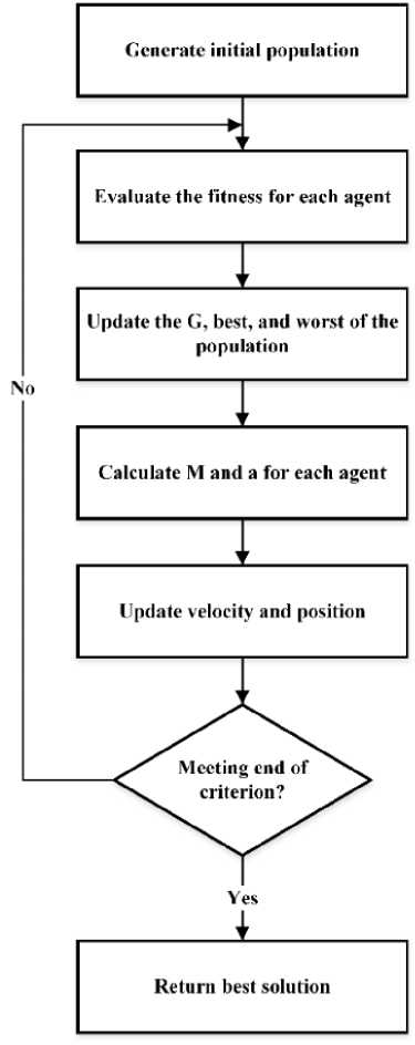
Figure 1. The Workflow of the Gravitational Search Algorithm
Table 1. GSA Parameters [31]
Parameters Values
An artificial neural network (ANN) is a kind of machine learning algorithm in which the workflow is inspired by the work of the nervous system. The smallest unit of the neural network is nerve cells (neurons). There are three basic sets of rules from the neuron model: multiplication, summation, and implementation of the activation function. The ANN process started from the input received by the neuron and the weight value of each available information. After entering the neuron, the
input values will be added by a summing function. Finally, the results will be converted by the activation function in each neuron. Then, the output will be sent to all neurons associated with it through the output weights. This process will be repeated on subsequent inputs.
Mathematically, ANN can be associated as a graph with neurons or nodes and synapses (edges). Hence, ANN operations are easily explained in linear algebraic notation. ANN architectures, such as single-layer feedforward networks (FFN), multi-layer FFN, lattice structures, and recurrent networks. The depth of ANN refers to the number of layers, while the width of ANN refers to the number of units in the layer. For example, a single-layer ANN is depicted in Figure 2.
Four ANN models were constructed by utilizing a different number of descriptors. We defined model 1, model 2, model 3, and model 4 comprised of 5, 6, 7, and 8 molecular descriptors. GSA performed the selection of the descriptor for each model. To improve the model's performance, the neural network parameter was optimized using a hyperparameter tuning procedure. The tuning procedure was performed by using grid search 5-fold cross-validation. The ANN parameters that are improved by the tuning scheme consist of hidden nodes, learning rates, momentum, and dropout rate. The range of the parameter values used in the turning scheme is provided in Table 2. We consider finding the optimal hidden node from the range values of 5 to 10 since the hidden node number is less than the input size. The learning rate and momentum utilized by the optimization algorithm are tuned with the range of values are 0.001 to 0.1 for the learning rate and 0.0 to 0.1 for momentum. To reduce the architecture complexity, we adjusted the dropout rate by using the range values from 0.0 to 0.2.
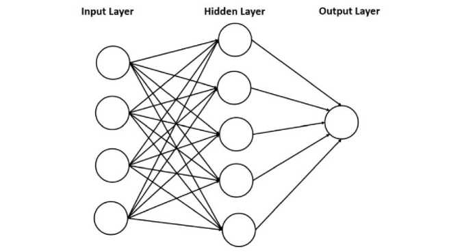
Figure 2. Single-layer Neural Network
Table 2. Parameters for Hyperparameter Tuning
|
Parameters |
Range |
|
Hidden node |
[5, 6, 7, 8, 9, 10] |
|
Learning rate |
[0.001, 0.01, 0.1] |
|
Dropout rate |
[0.0, 0.1, 0.2] |
|
Momentum |
[0.0, 0.1, 0.2] |
The performance of the models was determined by calculating several statistical parameters by using predicted values and the actual values. Several statistical parameters that represent the quality of the models are formulated as [32]:
r2 _ 1 [Sty—7i)(yi - y)]2
T 1
∑(yι- y)2 × ∑(yι - y)2
∩2 _ i _ ∑i=ι(yι- yι)2
q ∑"=1(yι-y)2
2-i_ ∑(yι-k ×yι)2
0 ∑(yι- y)2
, ∑(yι × yι)
∑(yι)2
,1 _ ∑(yι × yI)
∑(yι)2
t'o
2
— 1 —
∑Qi-k> ×yι)2
∑(yι-y)2
Tm2 — T2 × (1 — 7|T2 — To2|)
T'm — T2 × (1 — √T2 — T'2)
r2 _ {rm2+ r'm)
'm 2
τm — T2 (1 — √t2 — To2)
^^m — |Tm — Tm|
(14)
(15)
(16)
(17)
(18)
(19)
(20)
(21)
(22)
(23)
(24)
Where y and y represent the predicted and observed values of pKi, respectively, while y and y Represent the average predicted and observed values, respectively. The validity of a model is determined using the following threshold values [33]:
t2 > 0.6
Q2 > 0.5
r2
-
r2
< 0.1
0.85 ≤ ⅛ ≤ 1.15 or 0.85 ≤ ⅛' ≤ 1.15
∣To2 — t'o2∣ < 0.3 _
Ti > 0.5
∠lTm < 0.2
The applicability of the model against the train and test data was investigated by performing the applicability domain (AD) analysis. This analysis helps to interpret the model regarding the influence of descriptors in the prediction [34] and investigate the model's applicability against compounds in the data set. The AD definition is dependent on the model's descriptors and the experimental property [35]. AD is represented as a square region that determines the acceptability of data set prediction using the model [36]. In this study, AD was determined by using leverage approach, as formulated as:
H — X(XtX)-1Xt
(25)
Where X represents a descriptor matrix, the score matrix is constructed using the values of selected descriptors.
From 2904 descriptors, a set of molecular descriptors are selected by analyzing statistical parameter and performing GSA. In the first stage, the removal of descriptors with zero variance
decreased the descriptors numbers to 949. Then, the descriptor selection by using Pearson correlation analysis decreased to 61 of descriptors number.
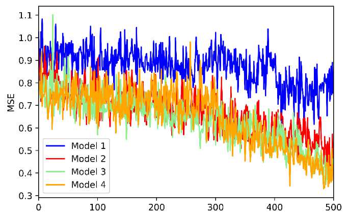
The selected molecular descriptors obtained from the statistical analysis are then further reduced by using GSA. In this stage, we performed four rounds of independent GSA to produce sets of the molecular descriptor with the number of the descriptors 5, 6, 7, and 8 used in four models, namely models 1, 2, 3, and 4, respectively. In the GSA process, the set of descriptors, or defined as a solution, was refined to obtain the solution with the lowest mean square error (MSE) value. The profile of MSE fluctuation during the iteration for four sets of descriptors was provided in Figure 3.
Iterations
Figure 3. The Plot of MSE during the Iteration of GSA
According to Figure 3, we found that the MSE of all models gradually decreases during the iteration. This indicates that the GSA scheme can solve with the lower MSE in the following iteration. Also, we found that the MSE for model 4, which comprised 8 descriptors, decreases faster than others. The order of model descriptors with respect to the decrease level of MSE is model 4, 3, 2, and 1, respectively. This points out that the descriptors number corresponds to the decreasing of MSE value during the GSA process. We summarized the molecular descriptor obtained from GSA for each model in Table 3, while the description of all selected descriptors is presented in Supporting Information [37], [38].
Table 3. Prediction Models and Their Molecular Descriptors
Model Total Selected Molecular Descriptors
Features
|
1 |
5 |
ATSC1dv, ATSC5d, SMR_VSA5, AATS6i.1, AATSC6m.1 |
|
2 |
6 |
ATSC1dv, ATSC1m.1, ATSC3i.1, AATSC7m.1, AATSC8v.1, VR2_Dzs |
|
3 |
7 |
ATSC1dv, AATS6v.1, AATS8i.1, AATSC3m.1, AATSC7m.1, AATSC8v.1, VR2_Dzs |
|
4 |
8 |
ATSC1dv, ATSC1d, ATSC5pe, EState_VSA2, AATSC7m.1, |
AATSC8v.1, VE3_Dzm.1, VR2_Dzs
The selected descriptor for all models found that the ATSC1dv descriptor is chosen for all models. This implies that the correlation between the descriptors and target variables is quite strong. Also, there are several selected descriptors in models 2 and 3, i.e., AATSC7m.1, AATSC8v.1, and VR2_Dzs. Those descriptors were also considered to influence the activity. By considering the type of selected descriptors, we found that almost all descriptors belong to the autocorrelation of
the topology structure. Here, autocorrelation is interpreted as a descriptor topology that encodes the molecular structure and physicochemical properties.
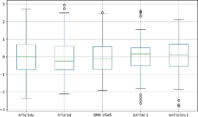
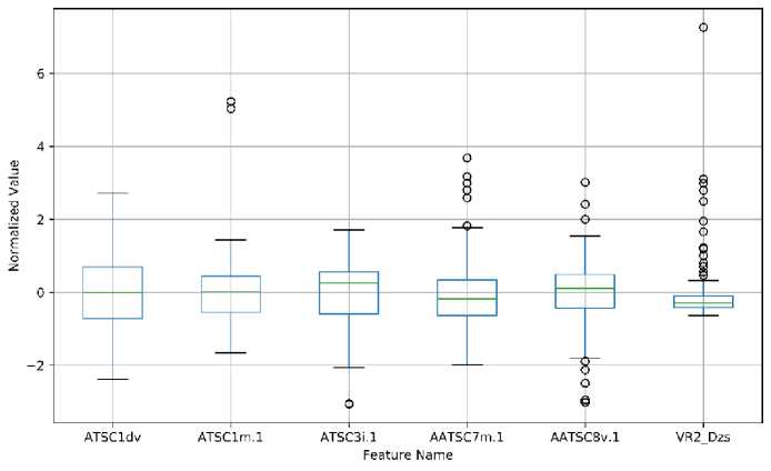
We analyzed the distribution of the selected descriptor by presenting the box plot of the normalized value of descriptors. The box plot of descriptors of models 1 and 2 is shown in Figure 4, while models 3 and 4 are available in Supporting Information. As for model 1, the distribution of all descriptors is quite similar. ATSC1dv parameter is found as the only descriptor without outliers data. As for model 2, the distribution of descriptor values varies with the range of VR2_Dzs is the smallest one. Also, many outliers data were found in AATSC7m.1, AATSC8v.1, and VR2_Dzs. As for model 3, VR2_Dzs is also the smallest range of descriptor values amongst the selected descriptors. Also, there are several descriptors with outliers data. As for model 4, the distribution of descriptor values is quite similar to model 3 with one descriptor.
OJ
Feature Name
(a)
(b)
Figure 4. The Boxplot Analysis of Descriptors used in (a) Model 1 and (b) Model 2
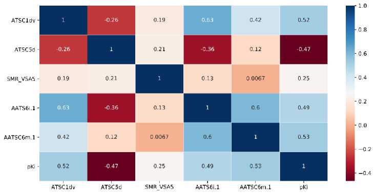
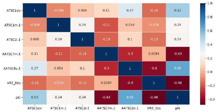
We also perform the correlation analysis to investigate the correlation between descriptors and target variables and amongst the descriptors. The correlation matrix of correlation is presented
as a correlation heatmap. For models 1 and 2, the heatmap is provided in Figure 5, while the heatmap for other models is available in Supporting Information.
(a)
(b)
Figure 5. The Heatmap Analysis of Descriptors used in (a) Model 1 and (b) Model 2
As for model 1, we found that ATSC1dv and AATSC6m.1 descriptors show a high correlation to the target with the correlations of 0.52 and 0.53, respectively. The high correlation of ATSC1dv to the target might be the reason for the appearance of the descriptor in all descriptor sets. Meanwhile, SMR_VSA5 shows the lowest correlation to the target with a correlation of 0.25. We also found a high correlation between ATSC1dv and AATS6i.1 descriptors with a correlation of 0.63. The high correlation corresponds to the similar type of those descriptors. As for model 2, the AATSC8v.1 descriptor shows the highest correlation to the target with a correlation of 0.65. Meanwhile, ATSC1m.1 and ATSC3i.1 present the lowest correlation to the target with the of 0.24. A high correlation amongst the descriptor was found between ATSC1dv and AATSC8v.1 with a correlation of 0.37.
As for model 3, the descriptor with the highest correlation to the target is also AATSC8v.1, as also found in model 2. This indicates that the parameters give a significant contribution to the model. Meanwhile, AATS8i.1 shows the lowest correlation to the target with a correlation of 0.35. The high correlation amongst the descriptor found between ATSC1dv and AATS8i.1 with a correlation of 0.59. As for model 4, AATSC8v.1 also shows the highest correlation to the target, while VE3_Dzm.1 shows the lowest correlation to the target with a correlation of -0.23. A high
correlation amongst the descriptors was found between ATSC1dv and Estate_VSA2, with a correlation of 0.41.
We found that the correlation of ATSC1dv with other selected topological descriptors is relatively high from the selected descriptor. This indicates that ATSC1dv represents the characteristic of those topological descriptors. Also, we found that AATSC8v.1 and VE3_Dzm.1 show the highest and lowest correlation, respectively, to the target amongst the selected descriptor.
The improvement of model performance was acquired by adjusting ANN parameters through the hyperparameter tuning scheme. The best parameters for each model were obtained from the tuning process, in which the parameters are listed in Table 4. We found that the optimized learning rate and momentum for all models are similar. Meanwhile, the optimized value of the hidden node and dropout rate of model 1 and model 2 are similar. This indicates that the character of the ANN architecture of both models is quite similar. However, we do not found any tendency regarding the optimized value of ANN parameters. This is related to the random factor involved in the model development of ANN.
|
Table 4. The Best Parameters of ANN Obtained from Hyperparameter Tuning | ||||
|
Parameters |
Model 1 |
Model 2 |
Model 3 |
Model 4 |
|
Hidden Node |
9 |
9 |
8 |
10 |
|
Momentum |
0.0 |
0.0 |
0.0 |
0.0 |
|
Learning Rate |
0.001 |
0.001 |
0.001 |
0.001 |
|
Dropout Rate |
0.1 |
0.1 |
0.0 |
0.0 |
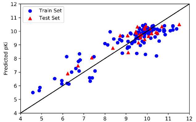
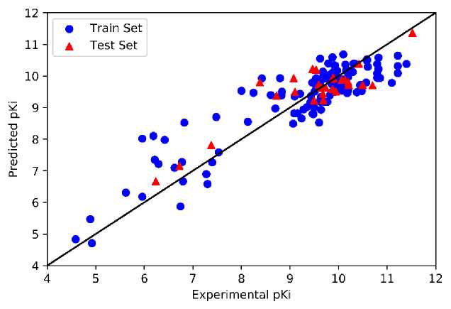
We implemented the optimized parameter in developing the ANN models to predicted pKi values. The plot of predicted and experimental values of pKi obtained by models 1 and 2 are presented in Figure 6, while the plot of those obtained by models 3 and 4 are shown in Supporting Information. We found that most train and test data points of all models close to the straight reference line with low deviation.
Experimental pKi
(a)
(b)
Figure 6. The Plot of Experimental pKi vs. Predicted pKi Obtained from (a) Model 1 and (b)
Model 2
Several validation parameters were calculated to determine the quality of models. First, we presented the validation parameter for the train and test set in Tables 5 and 6, respectively. By comparing those values with the threshold, we found that all models are valid and acceptable. However, we also utilized the parameters to determine the best model. As for the validation of the train set, we found that model 3 gives the best performance with the r2 and Q2 values are 0.84 and 0.81, respectively. Meanwhile, the worst performance was obtained from model 2, with the f r2 and Q2 values are 0.79 and 0.69, respectively.
As for the validation of the test set, we found that model 3 and model 4 give the best performance with the values of r2 is 0.82. Meanwhile, model 1 present the worst validation parameter with the value of r2 is 0.74. Here, we consider the values of r2 of the train and test set and Q2 of the train set to determine the best model. According to the consideration, we found that model 3 performs better than other models. This result indicates that the descriptors number used in model 3 is the most suitable for this case. Also, the performance of model 3 is related to the quality of the descriptor combination obtained from the GSA scheme of feature selection.
|
Table 5. The Validation Parameters of Train Set | ||||
|
Parameter |
Model 1 |
Model 2 |
Model 3 |
Model 4 |
|
r2 |
0.80 |
0.79 |
0.84 |
0.81 |
|
Q2 |
0.72 |
0.69 |
0.81 |
0.69 |
|
k |
1.0026 |
1.0027 |
1.0017 |
1.0006 |
|
(r2 - r02) |
0.005 |
0.004 |
0.0003 |
1.57e-5 |
|
r2 | ||||
|
lr0 -r'2 |
0.08 |
0.08 |
0.04 |
0.039 |
|
^^^^^^^^^^^^^ rm |
1.04 |
1.04 |
1.17 |
1.14 |
|
^rm |
0.19 |
0.19 |
0.15 |
0.16 |
|
Table 6. The Validation Parameters of Test Set | ||||
|
Parameter |
Model 1 |
Model 2 |
Model 3 |
Model 4 |
|
r2 |
0.74 |
0.75 |
0.82 |
0.82 |
|
k |
1.0029 |
1.0029 |
1.0018 |
1.0039 |
|
(r2 - r2) r2 |ro2 -r'2 |
0.034 |
0.017 |
0.002 |
0.004 |
|
0.24 |
0.17 |
0.56 |
0.071 | |
|
^^^^^^^^^^^^^ rm |
0.82 |
0.90 |
1.11 |
1.07 |
|
^r^ |
0.28 |
0.24 |
0.17 |
0.17 |
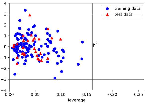
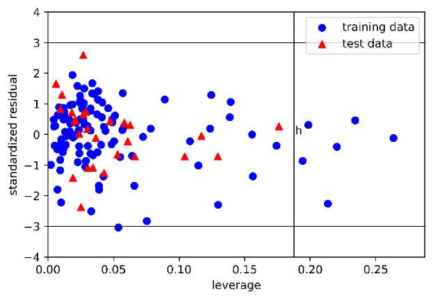
Furthermore, we investigated the applicability domain (AD) of each model by using a Williams plot. The AD plot of models 1 and 2 are presented in Figure 7, while the plot of models 3 and 4 are shown in Supporting Information. We found that h* values are different for each model. As for model 1, we found that only one train data lay outside the region with the standardized residual higher than the threshold. We also found that all of the test data lay inside the region. As for model 2, we found six train data points outside the region with leverage values higher than the h* value. However, there is no test data that is located outside the region.
As for model 3, three train data points outside the region with the leverage values are higher than h*, while all test data lie inside the region. As for model 4, we found two train data points and one test data point outside the region. Generally, even though several train data points are located outside the region, all models are still acceptable regarding the values of the validation parameter. Also, since all test data points are found inside the region, except model 4, we can point out that the prediction of the test set is reliable. The acceptability of this model highlight the ability of this model in predicting the activity of hydroxyethylamines compound outside the train data. By comparing the r2 score, we highlight that model 3 performs better than the previous study [18].
(a)
(b)
Figure 7. The Williams Plot of Applicability Domain Obtained from (a) Model 1 and (b) Model 2
Based on the results, the descriptor selection used in the QSAR model for predicting HIV-1 protease inhibitors activity was successfully performed by using the Gravitational Search Algorithm method. The development of four QSAR models was completed using the Neural Network method by varying the number of descriptors. In addition, a hyperparameter tuning scheme is used to improve the model performance. According to the results, all of the models are found to be valid and acceptable. We also found that model 3 that containing 7 descriptors give the most satisfying results with the values of r2 of the train and test set are 0.84 and 0.82, respectively, and the value of Q2 of the train set is 0.81. The analysis regarding the applicability domain indicates that the prediction of the test set by using model 3 is reliable. Since the validity of obtained QSAR model has been confirmed, we can use the model in virtual screening to filter HIV-1 protease inhibitors from the drug database.
References
-
[1] HIV.gov, "What Are HIV and AIDS?," HIV.gov, Jun. 17, 2019. https://www.hiv.gov/hiv-basics/overview/about-hiv-and-aids/what-are-hiv-and-aids (accessed Sep. 05, 2019).
-
[2] P. M. Sharp and B. H. Hahn, "Origins of HIV and the AIDS Pandemic," Cold Spring Harbor Perspectives Medicine, vol. 1, pp. a006841–a006841, 2011, doi:
10.1101/cshperspect.a006841.
-
[3] GHO, "Number of deaths due to HIV/AIDS - Estimates by WHO region," GHO Data Repository. http://apps.who.int/gho/data/node.main.623?lang=en (accessed Sep. 09,
2019).
-
[4] Y. Wang, Z. Lv, and Y. Chu, "HIV protease inhibitors: a review of molecular selectivity and toxicity," HIVAIDS - Research and Palliative Care, vol. 7, p. 95, 2015, doi:
10.2147/HIV.S79956.
-
[5] A. Brik and C.-H. Wong, "HIV-1 protease: mechanism and drug discovery," Organic & Biomolecular Chemistry, vol. 1, pp. 5–14, 2003, doi: 10.1039/b208248a.
-
[6] Hospital Care for Children, "8.2 Pengobatan Antiretroviral (Antiretroviral therapy = ART) ICHRC," Hospital Care for Children. http://www.ichrc.org/82-pengobatan-antiretroviral-antiretroviral-therapy-art (accessed Sep. 09, 2019).
-
[7] E. Estrada, "On the Topological Sub-Structural Molecular Design (TOSS-MODE) in QSPR/QSAR and Drug Design Research," SAR & QSAR Environmental Research, vol. 11, pp. 55–73, 2000, doi: 10.1080/10629360008033229.
-
[8] A. P. Asmara, “Studi Qsar Senyawa Turunan Triazolopiperazin Amida Sebagai Inhibitor Enzim Dipeptidil Peptidase-IV (DPP IV) Menggunakan Metode Semiempirik AM,” Berkala Ilmiah MIPA, vol. 23, p. 9, 2013.
-
[9] I. Kurniawan, D. Tarwidi, and Jondri, "QSAR modeling of PTP1B inhibitor by using Genetic algorithm-Neural network methods," Journal of Physics: Conference Series, vol. 1192, p. 012059, Mar. 2019, doi: 10.1088/1742-6596/1192/1/012059.
-
[10] I. Kurniawan, M. Rosalinda, and N. Ikhsan, "Implementation of ensemble methods on QSAR Study of NS3 inhibitor activity as anti-dengue agent," SAR & QSAR Environmental Research, vol. 31, no. 6, pp. 477–492, Jun. 2020, doi: 10.1080/1062936X.2020.1773534.
-
[11] I. Kurniawan, M. S. Fareza, and P. Iswanto, "CoMFA, Molecular Docking and Molecular Dynamics Studies on Cycloguanil Analogues as Potent Antimalarial Agents," Indonesian Journal of Chemistry, vol. 21, no. 1, Art. no. 1, Sep. 2020, doi: 10.22146/ijc.52388.
-
[12] H. F. Azmi, K. M. Lhaksmana, and I. Kurniawan, "QSAR Study of Fusidic Acid Derivative as Anti-Malaria Agents by using Artificial Neural Network-Genetic Algorithm," in 2020 8th International Conference on Information and Communication Technology (ICoICT), Jun. 2020, pp. 1–4, doi: 10.1109/ICoICT49345.2020.9166158.
-
[13] F. Rahman, K. M. Lhaksmana, and I. Kurniawan, "Implementation of Simulated AnnealingSupport Vector Machine on QSAR Study of Fusidic Acid Derivatives as Anti-Malarial Agent," in 2020 6th International Conference on Interactive Digital Media (ICIDM), Dec. 2020, pp. 1–4, doi: 10.1109/ICIDM51048.2020.9339632.
-
[14] V. Ravichandran, V. K. Mourya, and R. K. Agrawal, "Prediction of HIV-1 protease inhibitory activity of 4-hydroxy-5,6-dihydropyran-2-ones: QSAR study," Journal of Enzyme Inhibition and Medicinal Chemistry, vol. 26, pp. 288–294, 2011, doi: 10.3109/14756366.2010.496364.
-
[15] N. Saranya and S. Selvaraj, "QSAR Studies on HIV-1 Protease Inhibitors Using Non-Linearly Transformed Descriptors," Current Computer-aided Drug Design, vol. 8, pp. 10– 49, 2012, doi: 10.2174/157340912799218534.
-
[16] M. H. Fatemi, A. Heidari, and S. Gharaghani, "QSAR prediction of HIV-1 protease inhibitory activities using docking derived molecular descriptors," Journal of Theoretical Biology, vol. 369, pp. 13–22, 2015, doi: 10.1016/j.jtbi.2015.01.008.
-
[17] R. Darnag, B. Minaoui, and M. Fakir, "QSAR models for prediction study of HIV protease inhibitors using support vector machines, neural networks and multiple linear regression, " Arabian Journal of Chemistry, vol. 10, pp. S600–S608, 2017, doi:
10.1016/j.arabjc.2012.10.021.
-
[18] S. Bhargava, N. Adhikari, S. A. Amin, K. Das, S. Gayen, and T. Jha, "Hydroxyethylamine derivatives as HIV-1 protease inhibitors: a predictive QSAR modeling study based on Monte Carlo optimization," SAR & QSAR Environmental Research, vol. 28, no. 12, pp. 973–990, Dec. 2017, doi: 10.1080/1062936X.2017.1388281.
-
[19] I. I. Baskin, V. A. Palyulin, and N. S. Zefirov, "Neural Networks in Building QSAR Models," in Artificial Neural Networks, vol. 458, New Jersey: Humana Press, 2006, pp. 133–154.
-
[20] R. Guha and P. C. Jurs, "Interpreting Computational Neural Network QSAR Models: A Measure of Descriptor Importance," Journal of Chemical Information and Modeling, vol. 45, pp. 800–806, 2005, doi: 10.1021/ci050022a.
-
[21] A.-L. Milac, S. Avram, and A.-J. Petrescu, "Evaluation of a neural networks QSAR method based on ligand representation using substituent descriptors, " Journal of Molecular Graphics and Modelling, vol. 25, pp. 37–45, 2006, doi: 10.1016/j.jmgm.2005.09.014.
-
[22] S. Nagpal, S. Arora, S. Dey, and Shreya, "Feature Selection using Gravitational Search Algorithm for Biomedical Data," Procedia Computer Science, vol. 115, pp. 258–265, 2017, doi: 10.1016/j.procs.2017.09.133.
-
[23] S. A. Amin, N. Adhikari, S. Bhargava, T. Jha, and S. Gayen, "Structural exploration of hydroxyethylamines as HIV-1 protease inhibitors: new features identified," SAR & QSAR Environmental Research, vol. 29, pp. 385–408, 2018, doi:
10.1080/1062936X.2018.1447511.
-
[24] N. M. O'Boyle, M. Banck, C. A. James, C. Morley, T. Vandermeersch, and G. R. Hutchison, "Open Babel: An open chemical toolbox," Journal of Cheminformatics, vol. 3, p. 33, 2011, doi: 10.1186/1758-2946-3-33.
-
[25] H. Moriwaki, Y.-S. Tian, N. Kawashita, and T. Takagi, "Mordred: a molecular descriptor calculator," Journal of Cheminformatics, vol. 10, p. 4, 2018, doi: 10.1186/s13321-018-0258-y.
-
[26] C. W. Yap, "PaDEL-descriptor: An open source software to calculate molecular descriptors and fingerprints," Journal of Computational Chemistry, vol. 32, pp. 1466–1474, 2011, doi: 10.1002/jcc.21707.
-
[27] J. P. Papa et al., "Feature selection through gravitational search algorithm," in 2011 IEEE Int Conf Acoust Speech Signal Process (ICASSP), Prague, Czech Republic, 2011, pp. 2052–2055, doi: 10.1109/ICASSP.2011.5946916.
-
[28] "Newton’s law of gravitation,” Encyclopedia Britannica. Encyclopædia Britannica, inc., Accessed: Dec. 08, 2019. [Online]. Available: https://www.britannica.com/science/Newtons-law-of-gravitation.
-
[29] E. Rashedi, H. Nezamabadi-pour, and S. Saryazdi, “GSA: A Gravitational Search Algorithm,” Information Science, vol. 179, pp. 2232–2248, 2009, doi:
10.1016/j.ins.2009.03.004.
-
[30] E. Rashedi, H. Nezamabadi-pour, and S. Saryazdi, “BGSA: binary gravitational search algorithm,” Natural Computing, vol. 9, pp. 727–745, 2010, doi: 10.1007/s11047-009-9175-3.
-
[31] A. M. Al-Fakih, Z. Y. Algamal, M. H. Lee, M. Aziz, and H. T. M. Ali, “A QSAR model for predicting antidiabetic activity of dipeptidyl peptidase-IV inhibitors by enhanced binary gravitational search algorithm,” SAR & QSAR in Environmental Research, vol. 30, no. 6, pp. 403–416, Jun. 2019, doi: 10.1080/1062936X.2019.1607899.
-
[32] B. Sepehri and R. Ghavami, “Design of new CD38 inhibitors based on CoMFA modeling and molecular docking analysis of 4‑amino-8-quinoline carboxamides and 2,4-diamino-8-quinazoline carboxamides,” SAR & QSAR in Environmental Research, vol. 30, pp. 21–38, 2019, doi: 10.1080/1062936X.2018.1545695.
-
[33] A. Golbraikh and A. Tropsha, “Beware of q2!,” Journal of Molecular Graphics and Modelling, vol. 20, no. 4, pp. 269–276, Jan. 2002, doi: 10.1016/S1093-3263(01)00123-1.
-
[34] S. C. Peter, J. K. Dhanjal, V. Malik, N. Radhakrishnan, M. Jayakanthan, and D. Sundar, “Quantitative Structure-Activity Relationship (QSAR): Modeling Approaches to Biological Applications,” in Encyclopedia of Bioinformatics and Computational Biology, Elsevier, 2019, pp. 661–676.
-
[35] J. F. Aranda, D. E. Bacelo, M. S. L. Aparicio, M. A. Ocsachoque, E. A. Castro, and P. R. Duchowicz, “Predicting the bioconcentration factor through a conformation-independent QSPR study,” SAR & QSAR in Environmental Research, vol. 28, pp. 749–763, 2017, doi: 10.1080/1062936X.2017.1377765.
-
[36] P. Gramatica, “Principles of QSAR models validation: internal and external,” QSAR & Combinatorial Science, vol. 26, pp. 694–701, 2007, doi: 10.1002/qsar.200610151.
-
[37] “Descriptor List — mordred 1.2.1a1 documentation.” https://mordred-
descriptor.github.io/documentation/master/descriptors.html (accessed Jan. 08, 2020).
-
[38] DEDUCT, “Database of Endocrine Disrupting chemicals and their Toxicity profiles.” https://cb.imsc.res.in/deduct/descriptors/eJaFhpFsbWo (accessed Nov. 24, 2019).
77
Discussion and feedback