Spatial Based Deep Learning Autonomous Wheel Robot Using CNN
on
LONTAR KOMPUTER VOL. 11, NO. 3 DECEMBER 2020
DOI : 10.24843/LKJITI.2020.v11.i03.p05
Accredited B by RISTEKDIKTI Decree No. 51/E/KPT/2017
p-ISSN 2088-1541
e-ISSN 2541-5832
Spatial Based Deep Learning Autonomous Wheel Robot Using CNN
Eko Wahyu Prasetyoa1, Hidetaka Nambob2, Dwi Arman Prasetyaa3, Wahyu Dirgantaraa4, Hari Fitria Windi a5
aTeknik Elektro, Universitas Merdeka Malang
Jalan Terusan Dieng No. 62-64 Malang, Jawa Timur, Indonesia
1prasetyoekowahyu7@gmail.com;3arman.prasetya@unmer.ac.id;
4wahyu.dirgantara@unmer.ac.id; 5harry.fw@unmer.ac.id;
b Artificial Intelligence, Kanazawa University Kakumamachi, Kanazawa, Ishikawa, Jepang 2nambo@blitz.ec.t.kanazawa-u.ac.jp;
Abstract
The development of technology is growing rapidly; one of the most popular among the scientist is robotics technology. Recently, the robot was created to resemble the function of the human brain. Robots can make decisions without being helped by humans, known as AI (Artificial Intelligent). Now, this technology is being developed so that it can be used in wheeled vehicles, where these vehicles can run without any obstacles. Furthermore, of research, Nvidia introduced an autonomous vehicle named Nvidia Dave-2, which became popular. It showed an accuracy rate of 90%. The CNN (Convolutional Neural Network) method is used in the track recognition process with input in the form of a trajectory that has been taken from several angles. The data is trained using Jupiter's notebook, and then the training results can be used to automate the movement of the robot on the track where the data has been retrieved. The results obtained are then used by the robot to determine the path it will take. Many images that are taken as data, precise the results will be, but the time to train the image data will also be longer. From the data that has been obtained, the highest train loss on the first epoch is 1.829455, and the highest test loss on the third epoch is 30.90127. This indicates better steering control, which means better stability.
Keywords: Autonomous Wheel Robot, Nvidia, Artificial Intelligent, Convolutional Neural Network, Jupiter Note Book
Currently, the development of robotics is increasingly sophisticated, e.g., the use of a Preprepared trajectory on the Autonomous Wheel Robot. Furthermore, the Pre-prepared trajectory includes Artificial Intelligence (AI) [1] in the wheeled robot control system; therefore, it can move automatically. AI robot that was previously moving conventionally or driven by humans has started to be able to move automatically in this stage the robot can already be said machine learning. Machine learning and Artificial Intelligent have a difference where AI aims to increase the chances of success and not the accuration, while Machine Learning(ML) focuses on improving efficiency and no matter the success. AI's goal is to simulate natural intelligence in solving complex problems, whereas ML's goal is to learn from data to maximize machine performance[2]. AI is about making decisions, while ML allows systems to learn new things from data. AI will create systems to mimic humans and respond and behave accordingly. Other ML discs are involved in creating algorithms for self-learning.
In previous research, [3] developed an autonomous wheel robot using Raspberry Pi3 as a mini PC to process the data resource. It is used because it has a low price, but sometimes packet loss appears during the transmission data process in real-time because the ram is only 1 GB. Despite having a higher price, Nvidia Jetson Nanobot is equipped with an 8 GB ram, so the probability of
packet loss is smaller. In addition, the GPU owned by Nvidia also supports data image processing, so it can be processed faster.
The data that has been input and processed by the machine passes through two or more layers [4]. When more layers are used, the accuracy rate will also be increase [5]. This layer is a substitute for humans to make decisions independently without human assistance. One method of Deep learning is the Convolutional Neural Network or commonly abbreviated as CNN [6]. The CNN works by scan each section in the data to be used as a node. Each number in nodes is the result of matrix calculation. The robot can follow the track avoiding obstacles and doing work more efficiently and optimally.
Research related to autonomous driving in Artificial Intelligence laboratories has been done before [7], by simulating it using a program called the Carla simulator. It's an open-source one for autonomous car driving. Aims to continue the development to the next stage, this research focuses on making a prototype of an autonomous car that has three wheels; two regular wheels and one Omni wheel. The body is made of abs filaments that are printed using a 3D printer, the camera module as a place to pick up objects on the front. Thus the robot is expected to be able to operate on the ground, reading the area of the path and obstacles obtained through camera capture.
The method used in this study is the Resnet model of convolutional neural network (CNN) as follows :
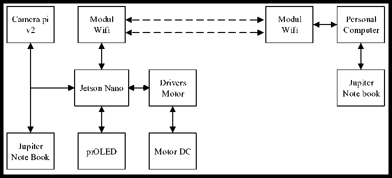
Figure 1. Design of research system developed
The design of the research system developed is illustrated in Figure 1. The camera retrieves digital imagery data passed to Nvidia Jetson Nanobot for processing, data from the received digital imagery will be processed with Nvidia Jetson Nanobot using Convolutional Neural Network method, this method is used to detect image data and train it, but this process is done separately in Personal Computer using Jupiter lab.
After Nvidia Jetson nano does training on the data that has been taken, the data will be reused as a reference to control the motor drivers who drive dc motors as actuators.
In the deep learning method, it is necessary to address significant problems in statistical machine learning [8]. The selection of a feature space that fits the representation learning approach becomes a problem in machine learning because the input space can be mapped to intermediate features. Deep neural networks have some difficulties [9], especially with high dimensional input spaces, e.g., images. This problem then encourages researchers to adopt a deep architecture, consisting of several layers with non-linear processing to solve the problem. Although there is already evidence of a successful case of a shallow network [10][11], the researchers found that
curse dimensionality becomes a problem in the case of multiple functions. Also, it was found that increasing the number of layers in the neural network can reduce the impact of backpropagation on the first layer. The descent of the gradient then tends to stop within the local minima or plateaus. However, this problem was solved in 2006 [12][13] through the introduction of layerwise unattended pre-training. In 2011, the Graphics Processing Unit (GPU) speed increased significantly, which made it possible to train Convolutional Neural Networks based architectures. Alexnet is won international competitions in 2011 and 2012. Then, in the following order of the following year, with the advancement of CPU and GPU, Deep learning and more for data-hungry deep learning techniques. The training and validation of motor sensor control models for urban driving in the real world were beyond the reach of most of the research groups [14]. Therefore, simulation testing is an alternative that can be done.
The result of cross multiplication Feedforward neural networks or Multilayer Perceptrons (MLPs) [15] are the base of the Deep Learning Model. The main objective of the feed-forward network is to define the mapping of input x to y,y-f (x; 0) categories and to estimate the value of the parameter θ, which is the result of the best function estimate [16][17].
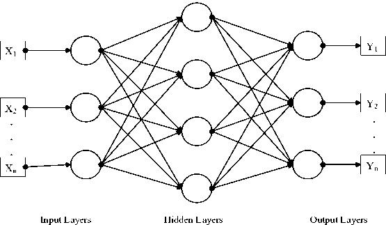
Figure 2. Example of MLPs With Hidden Layer
A feed-forward neural network has a structure consisting of many different functions. For example, Figure 2 consists of three different layer functions f(1),f(2),dan f(3) , forming. f(x) = f (3)(f(2) (f W (χ))))For this case, f (1) referred to as the input layer, f (2) is the second layer, or the hidden layer, and then f (3) is the output layer referred to in Figure 2. The overall length of the chain is the depth of the model. From here, this process is called Deep Learning [18].
This can provide a feed-forward network as a transformation of a linear function x into a nonlinear function of x, or it can be expressed as φ (x), where φ is a non-linear transformation. So it can be said that φ has a feature that describes x or provides a new representation of x. There are three general approaches [18]used to select φ mapping. That is:
-
a. Very generic based φ approach.
-
b. Manually engineered φ.
-
c. Parametrization of φ with a representation of φ(x; θ).
The last third option uses the feed-forward network as an application to study deterministic mapping, stochastic mapping, functions with feedback, and probability distributions on a single vector [18]. Most of the Neural Network models are designed using this principle.
CNN, introduced by LeCun, is mainly used to process data with a grid-like topology. It is simply neural networks that use convolutions instead of general multiplication. Usually, a convolutional network is composed of three-phase. The first phase, the convolutional layer, carries out convolution to produce a series of linear activations. In the second phase, the convoluted features
undergo a non-linear activation function, eventually, through the merged layer, which is called the downsampled feature [9][10][21].
Input Layers
Hidden Layers
Output Layers
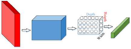
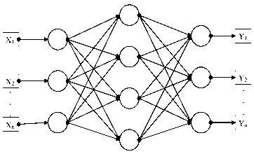
Figure 3. MLPs and CNN architecture
With the general availability of data and escalating computing power, deep learning approaches as convolutional neural networks (CNN), as evident, outperform traditional approaches.[22] CNN consists of multiple layers, each of which has an Application Program Interface (API) or commonly called a simple application program interface. In Figure 3, CNN, with the initial input of a threedimensional block, will be transformed into a three-dimensional output with several differentiation functions that have or do not have parameters. CNN forms its neurons into three dimensions (length, width, and height) in one layer. The proposed system performance was evaluated based on mean square error (MSE) [23][24].
In CNN, there are two main processes, namely Feature Learning and Classification
Feature Learning is the layers contained in Feature Learning, which is useful for translating input into features based on the characteristics of the input, which are in the form of numbers in vectors [25]. This feature extraction layer consists of a Convolutional Layer and a Pooling Layer.
-
a. Convolutional Layer will calculate the output of neurons connected to the local area in the input [26].
-
b. The Rectified Linear Unit (ReLU) will abolish off the lost gradient by adjusting the element activation function as f (x) = max f, 0 (0, x) [27] element activation will be performed when on the verge of 0. Advantages and disadvantages of using ReLU can expedite the Stochastic gradient compared with Sigmoid / tanh function, RelU is linear Not using exponential operations such as sigmoid / tanh, by creating an activation matrix when the threshold is 0. ReLU training is carried out it becomes fragile and dies, a large gradient that flows through ReLU causes weight updates, neurons are no longer active on the data point. If this happens, the gradient that flows through the unit will forever be zero from that point.
-
c. The pooling layer is a layer that reduces the dimensions of the feature map or better known as the step for down sampling [28], that speeds up computation. Fewer parameters need to be updated, and overfitting is overcome. Pooling that is commonly used is Max Pooling and Average Pooling. Max Pooling to determine the maximum value of each filter shift, while Average Pooling will determine the average value.
Classification This layer is useful for classifying each neuron that features extracted previously. Consists of:
-
a. Flatten is Reshape feature map into a vector, and then it can be used as input for the fully- connected layer [29].
-
b. Fully-connected The FC layer calculates the class score. Like a normal Neural Network and as the name suggests, every neuron in this layer will be connected to every number in the volume.
-
c. Softmax function calculates the probability of each target class over all possible target classes and will help to determine the target class for the input given. The advantage of using Softmax is that the probability of output ranges from zero to one, and the number of all probabilities will be equal to one. The softmax function used for the multiclassification model will return the probability that each class and the target class will have a high probability [30].
In the convolution layer, the convolutional algorithm converts the image into a vector without losing spatial information, which MLPs cannot do. Mathematically, the discrete convolution operation between two functions f and g, denoted by the operator *, can be defined as:
For a 2-dimensional image as input, the formula can be written as follows
(I*K)(i,j) = ∑N∑nKm,n)K(i + mJ + n)(2)
Since convolution is commutative, convolution can also be written as follows,
(K * MJ) = ∑N∑nKi + m,j + n)K(m,n)(3)
From these equations (1 and 2), I is a two-dimensional input, while K is a two-dimensional convolutional kernel.

Figure 4. 2D convolution between 3 x 4 input and 2 x 2 kernel
The principle of 2D convolution is to shift the convolutional kernel on the input. At each index position shown in Figure 3, element-wise multiplications are computed, they are summed. Then the result value is as follows:
q= a.m + b.n + e.o + f.p r = b.m + c.n +f.o + g.p s = cm + dn + go + gp
t = e.m + f.n + o.e + f.p u = f.m + g.n +j.o +k.p v = g.m + h.n + k.o +l.p
Refer to Figure 4, the kernel slides by the number of strides. This helps the user in downsampling the image. There is also a parameter called padding, which we can set up to control the size of the output.
This chapter will contain about testing the system on a device that is designed following the design to find out whether the tool is running as planned. Testing is carried out to compare the results of the theoretical design with the experimental results. From the test results.
The robots developed in this project are autonomous wheel robots that have three wheels, for more details can be seen in the following image.
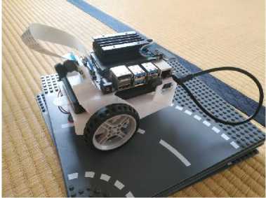
Figure 5 Autonomous wheel robot
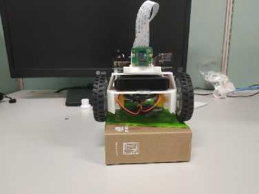
Figure 5 is a robot developed using three wheels, one of its wheels uses an Omni wheel that can move 360 degrees, and the other two wheels using conventional wheels connected to the DC motor as an actuator of the developed robot, in addition to being the robot's data receiver uses a camera on the front to capture the data received, for the brain to move the robot using NVidia Jetson Nanobot, to process data that has been stored using Convolutional Neural Network method (CNN) so that the robot can move smoothly along the track.
The camera used is the pi v2 camera module with the resolution used to capture images is 256 x 256 pixels, which serve as an image capture of objects with detailed and bright results. This camera device is a track detector or track that will be processed on the NVIDIA Jetson Nanobot.
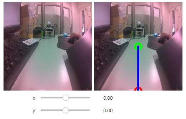
Figure 6. Display of Camera Testing at Jupiter Lab
Figure 6 Is a camera device that is connected to the Jetson Nanobot, which is placed on the front as a trajectory detector in the digital image camera testing device that is captured by this device, shown in Figure 6.
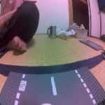
a b
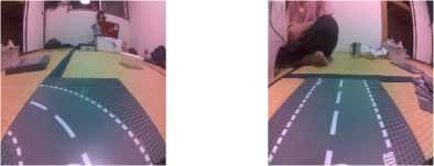
c d
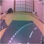
Figure 7. a, b, c, d, image display
Figure 7. (a) is the cut that is used, but this cut is only the right-turning part, Figure 7. (b) is the cut used this cut is only a straight section but takes half the angle of the whole track, Figure 7. (c) is the piece of track used but this track cut is only the left-turning part, Figure 7. (d) is the cut of the straight track taken from the end of the track to the last point of the track Display of the digital image captured by the camera as well as data to be processed using the Convolutional Neural Network method to Detect Pathways.
In this test, using CNN Resnet 34 method as described in the previous chapter in this process that determines how high the level of accuracy will be obtained in this research here is the training data process.
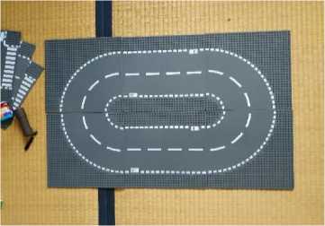
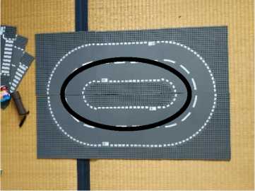
Figure 8. Track Used
Figure 8 shows a picture of the track used, after which the track is divided into parts. For example, see Figure 9.
a
b

c
d
Figure 9. a, b, c, d, The Marked Path
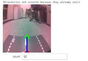
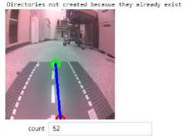
Figure 9. (a) is the cut that is used, but this cut is only the right turning part, Figure 9. (b) is the cut used, but this cut is only a straight section but takes half the angle of the whole track, Figure 9. (c) is the cut used but this cut is only the left turning part, Figure 9. (d) is a cut of a straight track taken from the end of the track to the last point of the track showing the result of the track that has been marked using the Jupiter Lab Note Book. The green pointer is the place where the track is marked as a point for Nvidia to make a decision.
Loss Function is a function in optimization problems to minimize the shortage or loss itself. The loss is damage or failure when training data, while the Number of Epoch is the number of a group of data repeatedly.
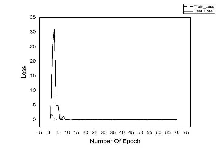
Figure 10. Function Loss Using Resnet 34
Figure 10. is a graph that shows the results of training data where training is carried out 70 times using the Resnet_34 Model, where the hidden layers used are 34 hidden layers, there is a comparison between training loss and test loss where if you want accurate accuracy results, the results of the test loss must be valuable equal to or higher than the training loss chart. It shows that for epoch less than ≤ 5, loss function obtained quite high with the peak point is around epoch = 3 and down monotone close to zero after passing epoch = 5.
|
Table 1. Loss Function Resnet 34 | ||
|
Epoch |
Train_Loss |
Test_Loss |
|
1 |
1.829455 |
0.432907 |
|
2 |
1.19932 |
24.971218 |
|
3 |
0.193119 |
30.90127 |
|
4 |
0.121705 |
4.869393 |
|
5 |
0.059956 |
4.776933 |
|
6 |
0.062019 |
0.30119 |
|
7 |
0.05823 |
0.198895 |
|
8 |
0.049085 |
1.056565 |
|
9 |
0.053102 |
0.051256 |
|
10 |
0.056029 |
0.036103 |
Based on Table 1. above, it can be seen that the highest Train Loss is in the first epoch with a value of 1.829455, while the highest Test Loss is in the third epoch with a value of 30.90127 while the epoch value is below the third epoch on an average value between 0.1 to 4.8. In previous research[31], using Carla to simulate how the CNN method works and obtained results training loss 0.00271 and validation loss 0.051. while the results of this study were obtained train loss 1.829455 and test loss 30.90127 this shows the results obtained in accordance with expectations. The value represents that, the model needs a more considerable amount of data so that train loss ~ test loss.
In this experiment, the Convolutional Neural Network deep learning method was used with the Resnet 34 models in the trajectory recognition process. To move smoothly, must take a picture of the trajectory from several angles not only take from one angle because the robot does not always move according to its path there must be a time when the robot moves out of the trajectory, and by the time it happens, the robot already has the data to make its own decision, the data image that has been stored next will be trained to get test loss and train loss values. From the data obtained, the highest train loss in the first epoch was 1.829455, and the highest test loss in the third epoch is 30.90127. The result obtained is then used by the robot to determine the path it will take. By adding the data, we want to train, we can reduce the level of loss that will be obtained, but the more data we train then, the longer it will take to train the data.
References
-
[1] D. A. Prasetya, P. T. Nguyen, R. Faizullin, I. Iswanto, and E. F. Armay, "Resolving the shortest path problem using the haversine algorithm," Journal of Critical Reviews, vol. 7, no. 1, pp. 62–64, 2020, doi: 10.22159/jcr.07.01.11.
-
[2] S. . Chang et al., "Resonant scattering of energetic electrons in the plasmasphere by monotonic whistler-mode waves artificially generated by ionospheric modification," Annales Geophysicae, vol. 32, pp. 507–518, 2014.
-
[3] M. G. Bechtel, E. McEllhiney, M. Kim, and H. Yun, "DeepPicar: A low-cost deep neural network-based autonomous car," Proc. - 2018 IEEE International Conference on Embedded and Real-Time Computing Systems and Applications(RTCSA 2018), pp. 11–21, 2019, doi: 10.1109/RTCSA.2018.00011.
-
[4] C. L. Zhang and J. Wu, "Improving CNN linear layers with power mean non-linearity," Pattern Recognition, vol. 89, pp. 12–21, 2019, doi: 10.1016/j.patcog.2018.12.029.
-
[5] D. A. Prasetya and I. Mujahidin, "2.4 GHz Double Loop Antenna with Hybrid Branch-Line 90-Degree Coupler for Widespread Wireless Sensor," in 2020 10th Electrical Power, Electronics, Communications, Controls and Informatics Seminar (EECCIS), Aug. 2020, pp. 298–302, doi: 10.1109/EECCIS49483.2020.9263477.
-
[6] J. Sun, Y. Fu, S. Li, J. He, C. Xu, and L. Tan, "Sequential human activity recognition based on deep convolutional network and extreme learning machine using wearable sensors," Journal of Sensors, vol. 2018, no. 1, 2018, doi: 10.1155/2018/8580959.
-
[7] W. Dharmawan and H. Nambo, "End-to-End Xception Model Implementation on Carla Self Driving Car in Moderate Dense Environment," AICCC 2019: Proceedings of the 2019 2nd Artificial Intelligence and Cloud Computing Conference, pp. 139–143, 2019, doi:
10.1145/3375959.3375969.
-
[8] Z. Q. Zhao, P. Zheng, S. T. Xu, and X. Wu, "Object Detection with Deep Learning: A Review," IEEE Transactions on Neural Networks and Learning Systems, vol. 30, no. 11, pp. 3212– 3232, 2019, doi: 10.1109/TNNLS.2018.2876865.
-
[9] A. R. Pathak, M. Pandey, and S. Rautaray, "Application of Deep Learning for Object Detection," Procedia Computer Science, vol. 132, no. Iccids, pp. 1706–1717, 2018, doi: 10.1016/j.procs.2018.05.144.
-
[10] N. Akhtar and A. Mian, "Threat of Adversarial Attacks on Deep Learning in Computer Vision: A Survey," IEEE Access, vol. 6, pp. 14410–14430, 2018, doi:
10.1109/ACCESS.2018.2807385.
-
[11] N. F. Ardiansyah, A. Rabi’, D. Minggu, and W. Dirgantara, “Computer Vision Untuk Pengenalan Obyek Pada Peluncuran Roket Kendaraan Tempur,” JASIEK (Jurnal Apl. Sains, Informasi, Elektron. dan Komputer), vol. 1, no. 1, 2019, doi: 10.26905/jasiek.v1i1.3142.
-
[12] H. Yu, D. C. Samuels, Y. yong Zhao, and Y. Guo, "Architectures and accuracy of artificial neural network for disease classification from omics data," BMC Genomics, vol. 20, no. 1, pp. 1–12, 2019, doi: 10.1186/s12864-019-5546-z.
-
[13] A. A. Elsharif, I. M. Dheir, A. Soliman, A. Mettleq, and S. S. Abu-naser, "Potato Classification Using Deep Learning," Advances in Animal Biosciences, vol. 3, no. 12, pp. 1–8, 2019.
-
[14] A. Dosovitskiy, G. Ros, F. Codevilla, A. Lopez, and V. Koltun, "CARLA: An Open Urban Driving Simulator," 1st Conference on Robot Learning (CoRL 2017), no. CoRL, pp. 1–16, 2017, [Online]. Available: http://arxiv.org/abs/1711.03938.
-
[15] W. Xiang, D. M. Lopez, P. Musau, and T. T. Johnson, "Reachable Set Estimation and Verification for Neural Network Models of Nonlinear Dynamic Systems," Safe, Autonomous and Intelligent Vehicles, pp. 123–144, 2019, doi: 10.1007/978-3-319-97301-2_7.
-
[16] A. A. Heidari, H. Faris, I. Aljarah, and S. Mirjalili, "An efficient hybrid multilayer perceptron neural network with grasshopper optimization," Soft Computing, vol. 23, no. 17, pp. 7941– 7958, 2019, doi: 10.1007/s00500-018-3424-2.
-
[17] W. A. H. M. Ghanem, A. Jantan, S. A. A. Ghaleb, and A. B. Nasser, "An Efficient Intrusion Detection Model Based on Hybridization of Artificial Bee Colony and Dragonfly Algorithms for Training Multilayer Perceptrons," IEEE Access, vol. 8, pp. 130452–130475, 2020, doi: 10.1109/access.2020.3009533.
-
[18] J. Heaton, "Ian Goodfellow, Yoshua Bengio, and Aaron Courville: Deep learning, " Genetic Programming and Evolvable Machines, vol. 19, no. 1–2, pp. 305–307, 2018, doi: 10.1007/s10710-017-9314-z.
-
[19] W. Dharmawan, "End-to-End Sequential Input with Time Distributed Model for Carla Self Driving Car in Moderate Dense Environment," 2019.
-
[20] C. Zhao, B. Ni, J. Zhang, Q. Zhao, W. Zhang, and Q. Tian, "Variational convolutional neural network pruning," 2019 IEEE/CVF Conference on Computer Vision and Pattern Recognition (CVPR), vol. 2019-June, pp. 2775–2784, 2019, doi: 10.1109/CVPR.2019.00289.
-
[21] Y. Liu, B. Fan, S. Xiang, and C. Pan, "Relation-shape convolutional neural network for point cloud analysis," 2019 IEEE/CVF Conference on Computer Vision and Pattern Recognition (CVPR), vol. 2019-June, pp. 8887–8896, 2019, doi: 10.1109/CVPR.2019.00910.
-
[22] A. Amidi, S. Amidi, D. Vlachakis, V. Megalooikonomou, N. Paragios, and E. I. Zacharaki, "EnzyNet: enzyme classification using 3D convolutional neural networks on spatial representation," Bioinformatics and Genomics, pp. 1–11, 2017.
-
[23] D. A. Prasetya, T. Yasuno, H. Suzuki, and A. Kuwahara, "Cooperative Control System of Multiple Mobile Robots Using Particle Swarm Optimization with Obstacle Avoidance for Tracking Target," Journal of Signal Processing, vol. 17, no. 5, pp. 199–206, 2013.
-
[24] A. P. Sari, H. Suzuki, T. Kitajima, T. Yasuno, and D. A. Prasetya, "Prediction Model of Wind Speed and Direction Using Deep Neural Network," JEEMECS (Journal of Electrical Engineering, Mechatronic and Computer Science), vol. 3, no. 1, pp. 1–10, 2020, doi: 10.26905/jeemecs.v3i1.3946.
-
[25] A. Dosovitskiy, J. T. Springenberg, M. Riedmiller, and T. Brox, "Discriminative unsupervised feature learning with convolutional neural networks," IEEE Transactions on Pattern Analysis and Machine Intelligence, vol. 1, no. January, pp. 766–774, 2014.
-
[26] S. Wang, J. Sun, I. Mehmood, C. Pan, Y. Chen, and Y. D. Zhang, "Cerebral micro-bleeding identification based on a nine-layer convolutional neural network with stochastic pooling," Concurrency and Computation Practice and Experience, vol. 32, no. 1, pp. 1–16, 2020, doi: 10.1002/cpe.5130.
-
[27] A. F. Agarap, "Deep Learning using Rectified Linear Units (ReLU)," Neural and Evolutionary Computing, no. 1, pp. 2–8, 2018.
-
[28] L. Jing, M. Zhao, P. Li, and X. Xu, "A convolutional neural network based feature learning and fault diagnosis method for the condition monitoring of gearbox," Measurement. Journal of the International Measurement Confederation (IMEKO), vol. 111, pp. 1–10, 2017, doi: 10.1016/j.measurement.2017.07.017.
-
[29] M. Yu et al., "Gradiveq: Vector quantization for bandwidth-efficient gradient aggregation in distributed CNN training," Advances In Neural Information Processing Systems 31 (NIPS 2018), vol. 2018-Decem, no. NeurIPS, pp. 5123–5133, 2018.
-
[30] S. Chen, C. Zhang, M. Dong, J. Le, and M. Rao, “Chen_Using_Ranking-CNN_for_CVPR_2017_paper.pdf,” Cvpr, pp. 5183–5192, 2017.
-
[31] C. Science, "End-to-End Spatial Based Deep Neural Network on Self-Driving Car," 2020.
177
Discussion and feedback