CHAOTIC OSCILLATIONOFA THREE-BUS POWER SYSTEM MODEL USING ELMANNEURAL NETWORK
on
LONTAR KOMPUTERVOL. 4, NO. 2,AGUSTUS 2013 ISSN: 2088-1541
Chaotic Oscillationofa Three-bus Power System Model Using ElmanNeural Network
I Made Ginarsa1, Adi Soeprijanto2, Mauridhi Hery Purnomo3
-
1Dept. of Electrical Engineering, Mataram University, Mataram
-
2Dept. of Electrical Engineering, Sepuluh Nopember Institute of Technology, Surabaya 3Dept. of Electrical Engineering, Sepuluh Nopember Institute of Technology, Surabaya e-mail: kadekgin@yahoo.com1, adisup@ee.its.ac.id2, hery@ee.its.ac.id3
Abstrak
Paper ini meneliti dan membahas secara mendalam mengenai osilasi chaotic pada sistem tenaga listrik.Dengan menggunakan sebuah three-bus pada sistem tenaga listrik, rute mungkin menyebabkan unjuk kerja chaotic sehingga dievaluasi, digambarkan serta dibahas dalam penelitian ini. Osilasi chaotic ini dimodelkan menggunakan Elmanneural network karena bentuknya yang sederhana dan juga melibatkan algoritmabackpropagation dengan adaptive learning rate dan momentumnya.Unjuk kerja learning rate dan momentumnya lebih baik dibandingkan jika tanpa momentumnya. Unjuk kerja chaotic dalam sistem tenaga listrik muncul karena sistem ini dioperasikan dalam mode critical. Unjuk kerja chaotic ini terdeteksi dengan munculnya sebuahchaotic attractordalam phase-plane trajectory.
Kata kunci:sistem tenaga listrik, Elman neural network, chaotic attractor, phase-plane trajectory
Abstract
Chaotic oscillation of power systems was deeply studied in this paper. By using a three-bus power system, route may cause chaotic behavior in power systems are evaluated, illustrated and discussed.Chaotic oscillationof power systems was modeled using Elman neural network because the Elman neural networkhas a simple form. Backpropagation algorithm with adaptive learning rate and momentum was proposed in this research. Performance of learning rate with momentum was better than learning rate without momentum. Chaoticbehaviors in a power system appeared due to the system operated in critical mode. A Chaotic behavior in power systems was detected by appearing a strange attractor (a chaotic attractor) in phase-plane trajectory.
Keywords:power systems, Elman neural network, chaotic attractor, phase-plane trajectory
model. The problem of controlled and suppressed of the presence of non-linear phenomena in power systems were addressed here in this paper. The bifurcation control approach is approach to modify the bifurcations and to suppress chaos [3,4]. The presence of chaos in a power system causing seriously unstable problem was studiedby Yu, et al.[5]. The existence chaos in power systems due to disturbing of energy at rotor speed has been found in Ref.[6]. One scheme of chaos utility was used on electrical systems for smelting which was based on chaos control. Lei et al. Demonstratedthat chaotic steel-smelting ovens regulate their heating current according to chaos control theory [7]. A control system using a neural network controller was presumed to be able to stabilize the unstable focus points of 2-dimensional chaotic systems; although, Konishiand Kokame stated that the control system did not require this presumption [8]. Elman neural network was used to predict short-term load forecasting in power systems [9]. Modeling of chaotic behavior using RNN has been studied in [10]. Various studies on controlling transient chaos have been carried out, such as those by Dhamala et al., and Dhamala and Lai attempted to control transient chaos in power systems using a data time series [11,12]. Strategies for controlling chaos in process plants have been tested on the Henon mapdiscrete chaotic system [13].
In this paper, we focused on the cause of chaotic oscillation in power systems and its model. By using Elman neural network model is proposed. The reason of using the Elman neural network because the Elman network is able to traindata both on present input and on past output, and other reason because an Elman RNN has simple form.
This paper is organized as follows: in advance, power system model used in this research is given in Section 2. Then, Elman neural network model isexplained in Section 3. Chaotic behavior due to sensitivityof initialcondition and analysis a chaotic behavior are presented in Section 4 and 5, respectively. The conclusionis given in the last section.
A Synchronous machine was modeled as a voltage (Eq0’) behind a direct reactance (xd’). The voltage magnitude was assumedas remaining constant at the pre-disturbance value, as shown in Fig.1(a).De Mello and Concordia as well as Padiyar and Kundur derivedof a machine connected toan infinite bus [13,14]. Meanwhile, if saturation and the stator resistance were neglected, the system condition was balanced with a static load. The mechanical mode block diagram of single-machine connected to infinite bus is shown in Fig.1(b).
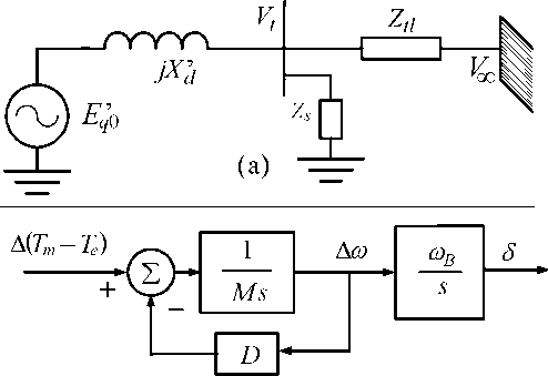
(b)
Figure 1.Single machine connected to infinite bus. (a) Circuit equivalent (b)Mechanical mode.
The machine wasconnected to infinite bus and supplied the load. Then the armature current flowedfrom the machine to the load. This current causedelectrical torque on the stator winding, and vice versa. The mechanical torque was produced by flux through the rotor winding. Meanwhile, whenthe rotor speed wasconstant, the rotor speed followed thesynchronous speed. When there was imbalanced energy, the rotor speed accelerated or decelerated and caused the swing equation.The swing equation is represented as follows:
Hδ+D ∆ω = Ta Tm Te
(1)
Where D, ∆ωare amping constant and rotor speed deviation, respectively. Eq.1 is a basic equation for mechanical modeof single machine connected to infinite bus. Furthermore,the the Eq. 1 can be expressed as follows:
δ = ωB ∆ω
(2)
∆d> = 1-(δTm -ΔTe D ∆ω)
M m e (3)
Where Δ Tm, ΔTe, δ, , D and M are mechanical torque, electrical torque, power angle, speed rotor, damping constant, inertia constant respectively.The system was developed from Ref.[3] and shown in Fig.3, which is regarded as one synchronous machine supplying power to a local dynamic load shunt with a capacitor (Bus 2) and connected by weak tie line to the extern system (Bus 3). The system equations are:
δ = ∆ω .
∆ω = 16.667 sin (^ L -5 + 0.087) VL
3.333.d.∆ω + 1.881
δL 496.872VL2
166.667 cos(δL -δ-0.087) VL
93.333VL (6)
666.667 cos (^L 0.209) VL
33.333Q1d + 43.333
VL 78.764 VL2
+ 26.217 cos (5 L -δ-0.012) VL
+14.523VL + 104.869 cos(5 L 0.135)
5.229Q1d 7.033
(4)
(5)
(7)
|
Table 1. Power system parameters | |
|
Y0 |
Ym θ0 θ m V0 Vm Pm M |
|
20. 0 |
5.0 5. 5. 1.0 1.0 1.0 0.3 0 0 |
|
D |
T C Kp a Kpv Kqω Kqv Kqv2 |
|
0.0 5 |
8.5 12. 0.4 0.3 0.0 2. 2.1 0 3 8 |
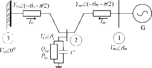
Figure 2.One line diagram power system with 3 buses.
δ, , d, Qld, δL,VL, arethe power angle, rotor speed deviation, damping constant, reactive load, voltage angle and magnitude at load bus, respectively. Eqs.4,5,6,and7 can be simplified into a uniform equation in Eq.8.
xf(x, 'O ,x ∈ Rn, λ ∈ Rp ,
(8)
Where x is vector state variables andλ is vector of parameters. The state variables are x = [ <5 , , <5L,VL]T, superscript T denote transpose of the associate vector.
Recurrent Elman network commonly is a two-layer network with feedback from the first-layer output to the first-layer input. This recurrent connection allows the Elman network to both detect and generate time-varying patterns. A two-layer Elman network is shown in Fig.3. The Elman network has tansig neurons in its hidden (recurrent) layer and purelin in its output layer. The Elman network differs fromconventional two-layer networks in that the first layer has a recurrent connection. The delay in this connection stores values from the previous time step, which can be used in the current time step. Thus, even if two Elman networks with the same weight and bias, are given identical inputs at a given time step, their outputs can be different due to different feedback states. Because network can store information for future reference, it is able to learn temporal pattern as well as spatial patterns [15,16,17,18]. The Elman network can be trained to respond and to generate, both kinds of patterns.
a1 (n) = tansig IW1,1 p + LW1,1a1
n 1 b1
(9)
a2 (n) = purelin LW2,1a1 n) + b2
The architecture 4:8:8:4 RNN is used in this research. Where p,a1(n), a2(n), IW1,1, LW1,1, LW1,2, b1 and b2 are the vector input, recurrent-layer output, purelin-layer output, weight first-layer, weight hidden layer back to first-layer, weight hidden layer to output layer and biases, respectively.
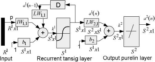
Figure 3.Elman recurrent neural network block diagram[18]
The RNN wastrained by using 1000 data points. Tansig and purelin activation function were used at hidden layer and at output layer, respectively. Data time series were obtained from the mathematical (exact) model in Eqs.4-7, respectively. The network performance is measured by mean square error (MSE). Formula of the MSE can be expressed by equation as follow:
MSE
1k -
k xˆ i
k i1
n
2
(10)
Where k, xn and xˆn are the size ofdata, input and estimation nth data.
Chaos definition and its properties have been given by Devaney and Alligood et al.[19,20]. Sensitivity of initial condition is one type of chaos properties. It is described by existing route to chaotic behavior in power systems caused by sensitivity of initial condition rotor speed (O)0). Initial rotor speed (ω0) in power systems was presented by disturbing ofenergy (DE). Kinetic energy disturbance was related to rotor speed deviation only. The large rotor speeddeviation was implemented as a large DE. When DE was smaller than the value of 1.3824 rad/s (ω0<1.3824 rad/s)a power system converged to a stable equilibrium point. When the DE was increased, the convergencebecame more difficult. At ω0 = 1.3825 rad/s, power systems produced route to a chaotic behavior in a longer time.When the DE was from1.3825 to 17003 rad/s, the final states were controlled by a chaotic behavior. Furthermore, while the DE excess than 1.7004 rad/s the system went to divergence or voltage collapse. Based on the simulation result it is shown that chaotic behavior in power systems due todisturbing of energy at the rotor speed deviation.
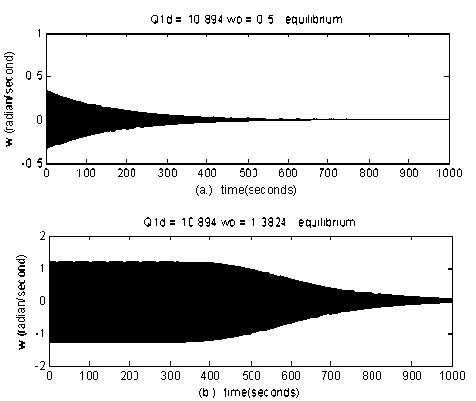
Figure 4.Simulation results with equilibrium point state
Table 2. System conditionwith different initial rotor speed (ω0)
|
ω0(rad/s) Times (s) |
Final state Time response |
|
0.5 1000 1.3824 1000 1.3825 1000 1.7003 1000 1.7004 10 |
Equilibrium point Fig.4(a) Equilibrium point Fig.4(b) Chaotic Fig.5(a) Chaotic Fig.5(b) Divergen - |
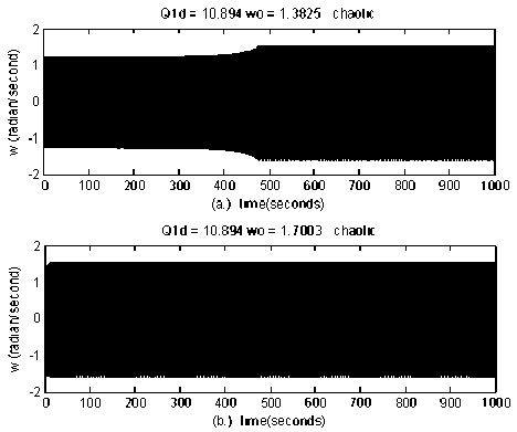
Figure 5.Simulation results with chaotic state
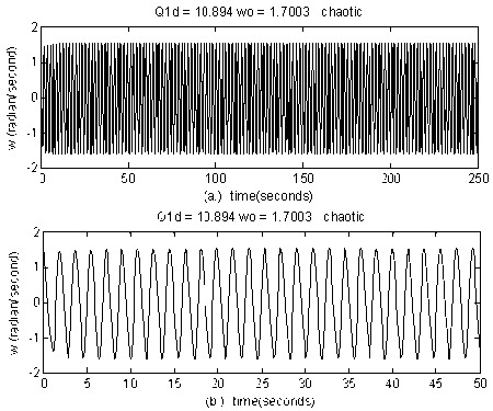
Figure 6. (a).Chaotic behavior of the rotor speed deviation (b). Magnified of Fig. 5 fromtime = 0 to time = 50 s
In this research, RNN initial simulation parameters were taken: learning rate train parameter = 0.17; increment learning rate = 1.2; decrement learning rate = 0.6; and momentum learning rate = 0.75. The training performance of RNN using adaptive learning rate and adaptive learning rate with momentum are listed in Table 3.The training process is organized as follows: performances (MSE) are obtained to 14.7001 X10 4 and 4.2209X10 4 at disturbance ω0 = 0.5 rad/s for algorithm backpropagation adaptive learning rate (traingda) and backpropagation learning rate algorithm with momentum (traingdx),respectively. Moreover,performances were obtained to 16.8361 ×10⁴ and 4.6115×10 4 at disturbance ω0 1.3825 rad/s. Furthermore, performances were obtained to 17.4185×10 4 and 4.9442×10 4at the disturbance ω0at the value of 1.7003 rad/s. During the training process the best performancewas obtained to 4.2209×10 4 at the disturbance of 0.5 rad/s.
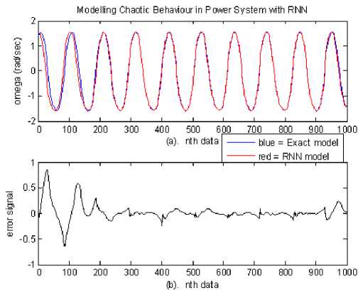
Figure 7. The chaotic behavior of the∆ωat ω0 =1.7003 rad/s
(a). Blue = exact model; red = RNN model (b). Error signal ofthe∆ω
Figs.7-9 show the time responses of an exact and Elman recurrent neural network (RNN) model. Fig.7(a) shows rotor speed deviation (∆ω) time response which was oscillated due to the disturbance occurred atω01.7003 rad/s. Rotor speed oscillations exist in range from 1.6052 to 1.5679 rad/s and from 1.511 to 1.6045 for the exact and RNN, respectively. Fig. 7(b) shows error signal of the rotor speed deviation; where the error signal is the difference of the exact and RNN model of the rotor speed deviation.
Voltage angle (δL) at Bus 2 is affected by disturbing of energy (DE) at generator bus (ω00.5 rad/s). The oscillation on voltage angle occurred at generator bus in a few second,then this oscillation decreased gradually and route to equilibrium point (fixed point) at point of 0.1128and 0.1116 rad for exact and RNN models, respectively. The error signal of the voltage angle was measured by mean square error (MSE = 3.8193%), and these results are shown in Table 4.
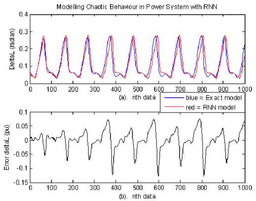
Figure 8.The chaotic behavior of the voltage angle when ω0 at 1.7003 rad/s. (a). Blue = exact; red = RNN (b). Error signal of the δL
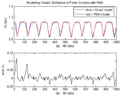
Figure 9. The voltage magnitude (VL) time response at co0 = 1.7003 rad/s (a). Blue = exact model; red = RNN model (b). Error signalof the VL
The voltage angle oscillation increased at the disturbance 1.3825, 1.600 and 1.7003 rad/s for exact model with amplitude in ranges (0.0600 to 0.1995 rad), (0.0351 to 0.2730rad), (0.0345 to 0.2748rad) and (0.0340 to 0.2756rad), respectively. And the oscillation for RNN model arefrom 0.0501 to 0.1879 rad, from 0.0460 to 0.2644rad, from 0.0332 to 0.2618radand from 0.0342 to 0.2613rad, respectively. This oscillation occurred in a longer time. Voltage angle time response occurring at disturbance co01.7003 rad/s can be shown in Fig. 8.
When the disturbance (ω0) at the value of 0.5 rad/s,the voltage magnitude oscillated in a few seconds. Furthermore, its decreased gradually route to equilibrium state (fixed point) at point 1.095 pu and 1.008 for exact and RNN model, respectively. By increasing disturbance at co 0 1.3824 rad/s voltage magnitude is oscillated in a longer time in ranges (0.9967 to 1.1207pu) and then amplitude reduced and fixed point at 1.1095 pu (1520 s).
On the opposite, when the disturbing of energy was increased up to 1.3825, 1.600 and 1.7003 rad/s, voltage magnitude oscillated for the exact model where the amplitude increased from0.8307 to 1.1220pu, from0.8285 to 1.1118puand from 0.8290 to 1.1119pu, respectively. And the oscillation for RNN model was in the ranges from 0.8497 to 1.1158pu, from 0.8580 to 1.1235puand from 0.8642 to 1.1185pu, respectively.In Fig.9, we can show that the voltage magnitude of the exact and RNN modelsexhibit chaotic behavior.
Table 3.Performance of training algorithm using learningrate momentum co0 Training Times (s) Performances
(rad/s) _________×102 MSE (×10-4)
|
traingda |
traingdx |
traingda |
traingdx | |
|
0.5 |
69.3861 |
37.403 |
14.7001 |
4.2209 |
|
1.3824 |
68.3250 |
42.342 |
17.2014 |
4.9080 |
|
1.3825 |
67.3329 |
36.750 |
16.8361 |
4.6115 |
|
1.7003 |
70.5781 |
41.840 |
17.4185 |
4.9442 |
State trajectory(orbit) of the Acoagainst δis shown in Fig.10, where many circlesare made by themselves with boundary ranges from 1.6011 to +1.5535 rad/sandfrom 0.1165 to +0.7583 rad for theco min- comaxandδ min- δmax, respectively. Thestate trajectoriesofthe RNN model are made in rangesfrom 1.6020 to +1.5524 rad/sandfrom 0.1145 to +0.7598 rad, respectively. The attractive form of the Aco-δis known as strange attractor (chaotic attractor).The strange attractorsof the δLagainstVLare shown in Fig.11. The strange attractor coordinateswere from 0.0345to 0.2748 rad and from 0.8285 to 1.1118pu for δ Lmax- δLmin and VLmax-VLmin, respectively.
Meanwhile, the RNN model of the <5L-VLwas from 0.0332to 0.2618 rad and from 0.8280 to 1.1235pu for <5Lmax- <5Lmin and VLmax-VLmin, respectively.
Table4.Power system state when variation of the DE was applied.
|
ω0&Model |
<5(rad) |
ω(rad/s) |
<5L (rad/s) |
VL (pu) |
|
0.5Exact |
eq 0.3095 |
osc 0.2104 to |
eq |
eq 1.095 |
|
0.2123 |
0.1128 | |||
|
RNN |
eq 0.3194 |
osc 0.2008 to |
eq |
eq 1.008 |
|
0.2010 |
0.1116 | |||
|
MSE (%) |
0.2636 |
11.1792 |
3.8193 |
8.7051 |
|
1.3824Exact |
osc 0.0245 |
osc 1.1546 to |
osc0.0600 to |
osc0.9967 to |
|
to 0.6160 |
1.1049 |
0.1995 |
1.1207 | |
|
RNN |
osc 0.0256 |
osc 1.0246 to |
osc0.0501 to |
osc0.9970 to |
|
to 0.6165 |
1.0049 |
0.1879 |
1.1135 | |
|
MSE (%) |
3.9625 |
6.3023 |
0.2040 |
0.1154 |
|
1.3425Exact |
osc 0.1156 |
osc 1.5711 to |
osc0.0351 to |
osc0.8307 to |
|
to 0.7578 |
1.5142 |
0.2730 |
1.1220 | |
|
RNN |
osc 0.1148 |
osc 1.5734 to |
osc0.0460 to |
osc0.8497 to |
|
to 0.7510 |
1.5165 |
0.2644 |
1.1158 | |
|
MSE (%) |
0.68 |
0.23 |
1.09 |
1.90 |
|
1.6000Exact |
osc 0.1165 |
osc 1.6011 to |
osc 0. 0345 |
osc 0.8285 to |
|
to 0.7583 |
1.5535 |
to 0. 2748 |
1. 1118 | |
|
RNN |
osc 0.1645 |
osc 1.6020 to |
osc0.0332 to |
osc0.8580 to |
|
to 0.7598 |
1.5524 |
0. 2618 |
1. 1235 | |
|
MSE(%) |
0.2163 |
2.8779 |
0.0460 |
0.0407 |
|
1.7003Exact |
osc .1157 to |
osc 1.6052 to |
osc 0. 0340 |
osc 0.8290 to |
|
0.7601 |
1.5679 |
to 0. 2756 |
1. 1119 | |
|
RNN |
osc 0.1345 |
osc 1.511 to |
osc 0.0342 to |
osc 0.8642 to |
|
to 0.7457 |
1.6045 |
0. 2613 |
1. 1185 | |
|
MSE(%) |
1.0522 |
17.8296 |
0.1284 |
0.1470 |
Note: eq = equilibrium point (fixed point); osc = oscillation.
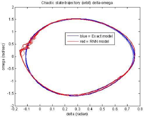
Figure 10. State trajectory of the ∆ω -δ when disturbance was applied at ω0 = 1.600 rad/s
Furthermore, existence of the chaotic attractors can also be depicted in Figs.12 and 13 for the ω01.7003 rad/s. Fig.12 was produced by the ∆ωagainstsδstate trajectories at coordinates from 1.6052 to +1.5679 rad/sandfrom 0.1157 to +0.7601 rad for the ω min- ωmax and δmin- δmax, respectively. The results of theRNN model are depicted by red circles at coordinates from 1.5110 to +1.6045 rad/sandfrom 0.1345 to +0.7457 rad for the ω min- ωmax and δ min- δ max, respectively.
Fig.13 shows the δLagainstVL state trajectories at coordinates from 0.0351to 0.2756 rad and from 0.8290 to 1.1119 pu for the δ Lmax- δLmin and the VLmax-VLmin, respectively. State trajectories of the RNN model can be depicted by red points at coordinates from 0.0342to 0.2613 rad and from 0.8642 to 1.1185 pu for theδLmax- δLmin and the VLmax-VLmin, respectively. The complete simulation results are tabulated in Table 4.
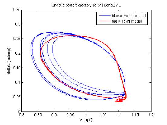
Figure 11. The δL-VL state trajectory when the DE at ω0 = 1.6 rad/s was applied
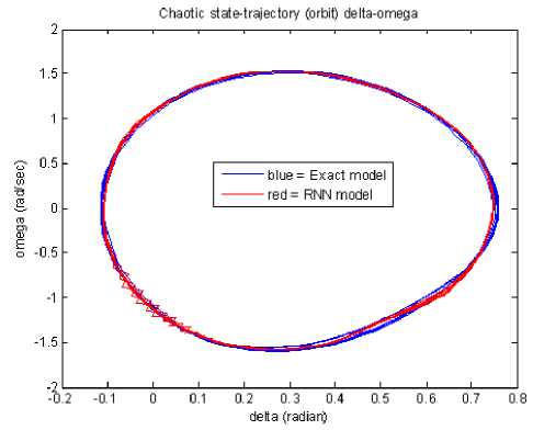
Figure 12. The ∆ω- state trajectory when the DE at the value of 1.7003 rad/s was applied to a power system
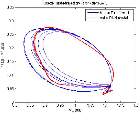
Figure 13. The <5L-VLstate trajectory when the DE at the value of 1.7003 rad/s was applied to a power system
Based on the in Table4that the largest MSE was 17.8296, where the largest MSE was obtained onthe speed rotor deviation (∆ω) at the value of 1.7003 rad/s. Simulation results show that chaotic behavior of power systems can be modeled by the Elman recurrent neural network.
Chaotic oscillationsin power systems using exact and RNN models are deeply studied in this research. The exact model was obtained using mathematical model. Then, the RNN model is obtained by training process using the data from exact model simulation. The training of the RNN model using adaptive learning rate both with and without momentum is compared. The performace of the adaptive learning rate with momentum is better than the other one. Chaotic behaviors are detected in power systems by appearing chaotic attractors both at power anglerotor speed and at magnitude-angle voltage state trajectories in phase-plane.
Chaotic behavior of power systems was an interest topic research in recent years. In the future, thechaotic behavior of power systems should be reduced and vanished by applying control strategy properly.
References
-
[1] H.-D.Chiang, et al, “On Voltage Collapse in Electric Power System”, IEEE Trans. on Power Syst., Vol. 5, No.2, May 1990.
-
[2] H.-D.Chiang,P.P. Varaiya, F.F. Wu and M.G. Lauby, “Chaos in a Simple Power System”, IEEE Trans. on Power Syst., Vol. 8, No. 4, November 1993.
-
[3] H.O.Wang, “Control of Bifurcation and Routes to Chaos in Dynamical System”, Thesis Report Ph.D, ISR, The University of Maryland, USA, 1993.
-
[4] H.O.Wang, E.H.Abedand A.M.A.Hamdan, Bifurcations, “Chaos and Crises in Voltage Collapse of a Model Power System”, IEEE Trans. on Circuit and Systems 1: Fundamental, Theory and Applications, Vol. 41, No.3, March 1994.
-
[5] Y.Yu, H.Jia, P.Li and J.Su, “Power System Instability and Chaos”, Elect. Power Syst. Res., Vol. 65, pp. 187-195, 2003.
-
[6] I M.Ginarsa, A.Soeprijanto and M.H. Purnomo, “Implementasi Model Klasik untuk Identifikasi Chaotic dalam Sistem Tenaga Listrik Akibat Gangguan Energi”, Procs.of the 9thSITIA, Surabaya, 2008.
-
[7] Z.-M.Lei,Z.-J. Liu, H.-X.Sun andH.-X. Liu, “Control and Application of Chaos in Electrical System”, Proceedings of the Fourth International Conference on Machine Learning and Cybernatics, Guangzhou, 18-21August 2005.
-
[8] K.Konishi and H. Kokame, “Stabilizing and Tracking Chaotic Orbits Using a Neural Network”, NOLTA’95, Las Vegas, USA, December 10-14, 1995.
-
[9] H. Su andY. Zhang, “Short-Term Load Forecasting Using H∞ Filter and Elman Neural Network”, Procs. Of IEEE ICCA, Guangzhou China, May 30 to June 1,2007.
-
[10] I M.Ginarsa, A.Soeprijanto and M.H. Purnomo, “Modeling of Chaotic Behavior Using Recurrent Neural Networks in Power Systems”, Procs. of ICACIA, Jakarta, 2008.
-
[11] M.Dhamala,Y.-C.Lai and E.J. Kostelich, “Analyses of Transient Chaotic Time-series”, Physical Review E, Vol. 64, 2001.
-
[12] M.Dhamala andY.-C.Lai, “Controlling Transient Chaos in Deterministic flows with Applications to Electric Power Systems and Ecology”, Physical Review E, Vol. 59, No.2, February 1999.
-
[13] J. Krishnaiah, C.S. Kumar and M.A. Faruqi, “Modelling and Control of Chaotic Processes through Their Bifurcation Diagrams Generated with The Help of Recurrent Neural Network Models: Part 1-Simulation Studies”, Journal of Process Control, Elsevier, 2006.
-
[14] K.R.Padiyar, “Power System Dynamic Stability and Control”, John Wiley & Sons (Asia) Pte Ltd, Singapura, 1984.
-
[15] P.Kundur, “Power System Stability and Control”, EPRI, McGraw-Hill, New York, 1994.
-
[16] O.M. Omidvar and D. L. Elliot, “Neural Systems for Control”, Academic Press, February 1997.
-
[17] L.R. MedskerandL.C. Jain, “Recurrent Neural Networks: Design and Applications”, CRC Press, Boca Raton, 2001.
-
[18] M. Norgaard, “Neural Network Based System Identification Toolbox: for Use with Matlab”, Department of Automation, Department of Mathematical Modeling, Technical University of Denmark.
-
[19] --------, “MATLAB Version 7.04: The Language of Technical Computing”, The Matworks
Inc, 2005.
-
[20] R.L. Devaney, “A First Course in Chaotic Dynamical Systems: Theory and Experiment”, Addison-Wesley Publishing Company Inc, New York, 1992.
255
Discussion and feedback