Comparison of K-Nearest Neighbor And Modified K-Nearest Neighbor With Feature Selection Mutual Information And Gini Index In Informatics Journal Classsification
on
p-ISSN: 2301-5373
e-ISSN: 2654-5101
Jurnal Elektronik Ilmu Komputer Udayana
Volume 10, No 3. February 2022
Comparison of K-Nearest Neighbor And Modified K-Nearest Neighbor With Feature Selection Mutual Information And Gini Index In Informatics Journal Classsification
Benedict Emanuel Sutrisnaa1, AAIN Eka Karyawatia2, Luh Arida Ayu Rahning Putria3, I Wayan Santiyasaa4, Agus Muliantara a5, I Made Widiarthaa6,
aProgram Studi Informatika, Fakultas Matematika dan Ilmu Pengetahuan Alam, Universitas Udayana 1benemanuel0805@gmail.com
Abstract
With the rapid development of informatics where thousands of informatics journals have been made, a new problem has occured where grouping these journals manually has become too difficult and expensive. The writer proposes using text classification for grouping these informatics journals. This research examines the combinations of two machine learning methods, K-Nearest Neighbors (KNN) and Modified K-Nearest Neighbors with two feature selection methods, Gini Index (GI) and Mutual Information (MI) to determine the model that produces the higherst evaluation score. The data are informatics journals stored in pdf files where they are given one of 3 designated labels: Information Retrieval, Database or Others. 252 data were collected from the websites, neliti.com and garuda.ristekbrin.go.id. This research examines and compares which of the two methods, KNN and MKNN at classifying informatics journal as well as determining which combination of parameters and feature selection that produces the best result. This research finds that the combination of method and feature selection that produces the best evaluation score is MKNN with GI as feature selection producing precision score, recall score and f1-score of 97.7%
Keywords: Text Classification, KNN, MKNN, Mutual Information, Gini Index, Informatics Journal.
The field of informatics is experiencing rapid development. Hundreds of research in various fields are conducted each year where their results would be used as material for future research. Though not all findings will be relevant towards a research that’s being conducted, as such it would be prudent to group those research to make it easier to find relevant references for future research. Unfortunately, the quick growth of informatics with hundreds of research being published each year makes grouping these research through human efforts near impossible and very expensive. This problem can be overcome with computers through text classifications.
According to [1] various classification methods can be used for document classification in various domains, such as digital libraries and scientific literature. According to [2] one algorithm that can solve the classification problem is K-Nearest Neighbor (KNN) which has an easy to understand and implement algorithm, however it has a weakness where larger dimensionality of data will negatively affect its performance. Several research have been made to overcome this problem, Research conducted by [3] found that feature selection improves the evaluation scores of KNN and Naïve Bayes compared to when both don’t use feature selection. [4] created a variant of KNN named Modified K-Nearest Neighbor which has a better evaluation score than KNN. However feature selection was not used in said research, thus it is not known how feature selection would affect its performance. According
to [5] the use of the feature selection method Mutual Information (MI) improves the evaluation score of the Support Vector Machine algorithm in classifying Indonesian news articles. [6] found that the Gini Index (GI) feature selection method increases the evaluation score of KNN in classifying cognitive level documents. Based on those sources, the writer believes that both feature selection methods can be used on informatics journals, but wants to know which method produces the highest evaluation score if only use one feature selection method.
Based on the existing problem and the related research of which are the basis of this research, the writer intends to compare KNN and MKNN with MI and GI as feature selection with the hopes that this research find the combination algorithm and feature selection with the highest evaluation score.
This research is divided in to two stages. In the first stage, models, which are combinations of algorithms and feature selection methods, are divided in to 3 categories based on which feature selection methods are used, namely: none, GI, and MI. The best model of each category is chosen to continue for the second stage. In the second stage, the 3 chosen models is tested again to determine the best model. Testing in this research is divided in to 2 phases, the training phase and the testing phase. The training phase is where training data is processed so that the model can use it in testing phase. It consists of preprocessing, TF-IDF weighting and feature selection. The testing phase is where the testing data is classified by the model and its results are evaluated. It consists of preprocessing, TF-IDF weighting, feature selection, classification, and evaluation.
Data is collected from 2 web sources, https://www.neliti.com/id/conferences/semnasif and https://garuda.ristekbrin.go.id/area. 252 information journals were collected and divided evenly in to 3 labels, Information Retrieval, Information and Database Systems and Their Applications, and others. Data labeling is done by the writer and evaluated by 12 fellow students from Text Mining and Big Data disciplines using the Kappa statistic.
Preprocessing aims to make the input documents more consistent to facilitate text representation, which is necessary for most text analytics task [1]. As can be seen in Figure 1, this research applies several preprocessing methods, namely case folding, punctuation removal, stemming, stop word removal and tokenization. Case folding is the process of converting letter in to the same case, particularly uppercase letters in to lowercase letters. Stop words removal is the removal of very common and low information words known as stop words. Stemming is the process of cutting inflected words in to their word stem. Tokenization is the process of dividing text in to several units called tokens, the tokens in this research consist of individual words.

Figure 1. Preprocessing
Term Frequency – Inverse Document Frequency (TF-IDF) is a composite weighting method for each tem in every document. TF-IDF assumes has a good class of distinction occurs if a term has high freqeuncy in one document and low frequency in other documents [2].
The following are the steps of TF-IDF, see Figure 2:
-
a. Calculate term frequency of term t in documet d (tft,d)
-
b. Calculate document frequency of term t (dft)
-
c. Calculate inverse document frequency
N
ιdft = log- (1)
aJt
With idft as the inverse document frequency of term t, df as the document frequency of term t, and N as the total number of documents
-
d. Calculate TF-IDF
‰ = ‰ × idft
(2)
With Wt,d as weight of term t in document d.

Figure 2. TF-IDF Weighting
Gini Index (GI) is a measurement of statistical dispersion intended to represent wealth distribution of a country developed by Corrado Gini. GI is often used to measure discriminative power in a feature. GI is typically used for categorical variables, but can be generalized to numeric attributes through discretization [7]. The GI formula is as follows:
GI(x) = 1-∑Y=1P(i)2
(3)
With Y as total labels, x as term, and p(i) as probability of term x in document labeled i.
The steps of Gini Index can be seen in Figure 3.

Figure 3. Gini Index
According to [8] mutual information (MI) is the measurement of the amount of information that one random variable contains about another random variable. MI is the reduction of uncertainty of a random variable caused by information from another random variable. MI determines the correlation between two words in a data set, if the MI score is large then the two terms often co-occur thus they relate semantically. Conversely a small MI score means that when one of them appears then the other does not, indicating no semantic relation. The formula for MI is as follows:
I(x,y) = ΣxEX∑yEγP(x.y)log (^yyy--)
(4)
With p(x,y) as joint probability of x and y, p(x) as probability of x, and p(y) as probability of y.
The steps of Mutual Information can be seen in Figure 4.

Figure 4. Mutual Information
K-nearest neighbours (KNN) locally determines the decision boundary (label). For 1NN, each document is inserted in to the label of its nearest neighbours. For KNN, each document is inserted in to the majority label of its k nearest neighbours, with k as a parameter. KNN classification is based on contiguity hypothesis, which assumes a document d has the same class as its neighbouring training document [2]. The following are the steps of KNN classification, with the flowchart shownin Figure 5: a. Determine the value of k.
-
b. Calculate the distance of the object with each data point. Calculation is done using Euclidian distance with the following formula:
D (x, y') = √∑t=1(xi - yi)2 (5)
With D as distance, and x and y as training data and testing data respectively.
-
c. Gather the data points with the smallest distance as many as k.
-
d. Determine the class majority of the gathered data points.

Figure 5. K-Nearest Neighbor
According to [4] Modified K-Nearest Neighbours (MKNN) is a variation of KNN which computes a kind of weight named validity on training data based on the number of same labeled neighbours divided by the total of neighbors. The following is the algorithm of MKNN, with the flowchart shown in Figure 6:
-
a. Determine the value of K.
-
b. Determine validity (v) for each training data with the formula:
v(x) = 1∑^=1^ (lbl(x),lbl(Nl(x)'))(6)
With the function S to calculate similarity between x and the ith nearest neighbour with the formula:
With H as the number of neigbors to calculate v, x as designated training data, lbl(x) as label of x, and Ni(x) as ith nearest neighbor of x
-
c. Calculate the weight of k nearest neighbor with the formula:
+ O ■ 5
With W(i) as weight of ith neighbour and d as Euclidean distance
-
d. Compute the sum weights of every neighbour according to their label.
-
e. Choose the label with the highest total weight.
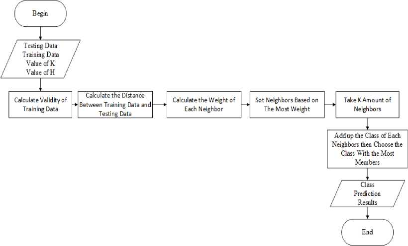
Figure 6. Modified K-Nearest Neighbor
Measurement of each model’s effectiveness in classification is done by using precision, recall and f1-score as evaluation scores. Precision is the ratio of total true positive to the sum total of true positive and false positive prediction. Recall is the ratio of total true positive to the sum total true positive and false negative prediction. F1-score is a calculation that combines precision and recall. The formula of precision, recall and f1-score is as the following.
TTP
TTP+TFP
TTP
TTP+TFN
2
1 ι 1
Precisian Recall
(9)
(10)
(11)
With:
-
• TTP is the total true positive prediction
-
• TFP is the total false positive
-
• TFN is the total false negative
The precision, recall and f1-score of each model is recorded and compared with emphasis on f1-score for deciding the best model.
The following are comparisons between KNN and MKNN with various parameters in 3 categories, without feature selection, with GI, and with MI. The best model of each category will be compared in the next round of testing.
Comparison of Models without Feature Selection
Table 1 is the evaluation result of KNN and MKNN without feature selection. The testing finds that KNN with the parameters k = 3 produced the best result with an f1-score of 25.1%
Table 1. Evaluation Results of Models without Feature Selection
|
Metode |
Precision (average) |
Recall (average) |
F1-score (average) | ||||||
|
k = 3 |
k = 5 |
k = 7 |
k = 3 |
k = 5 |
k = 7 |
k = 3 |
k = 5 |
k = 7 | |
|
KNN |
31.4% |
24.4% |
28.6% |
36.2% |
38.6% |
37.6% |
23.1% |
25.1% |
23.4% |
|
MKNN (h=10) |
11.1% |
11.1% |
11.1% |
33.3% |
33.3% |
33.3% |
16.7% |
16.7% |
16.7% |
|
MKNN (h=20) |
11.1% |
11.1% |
11.1% |
33.3% |
33.3% |
33.3% |
16.7% |
16.7% |
16.7% |
|
MKNN (h=30) |
11.1% |
11.1% |
11.1% |
33.3% |
33.3% |
33.3% |
16.7% |
16.7% |
16.7% |
Comparison of Models with GI
Table 2 is the evaluation result of KNN and MKNN with GI as feature selection. The testing finds that MKNN with the parameters k = 3 and h = 30 produced the best result with an f1-score of 95.5%.
Table 2. Evaluation Results of Models with GI
|
Metode |
Precision (average) |
Recall (average) |
F1-score (average) | ||||||
|
k = 3 |
k = 5 |
k = 7 |
k = 3 |
k = 5 |
k = 7 |
k = 3 |
k = 5 |
k = 7 | |
|
KNN |
95.0% |
93.8% |
93.8% |
94.9% |
93.7% |
93.6% |
94.9% |
93.3% |
93.3% |
|
MKNN (h=10) |
91.7% |
90.5% |
90.3% |
90.4% |
89.5% |
89.4% |
90.2% |
89.0% |
88.9% |
|
MKNN (h=20) |
93.6% |
92.4% |
92.2% |
94.3% |
93.3% |
93.3% |
94.0% |
92.4% |
92.2% |
|
MKNN (h=30) |
95.8% |
95.2% |
95.2% |
95.4% |
94.8% |
94.7% |
95.5% |
94.8% |
94.7% |
Comparison of Models with MI
Table 3 is the evaluation result of KNN and MKNN with MI as feature selection. The testing finds that MKNN with the parameters k = 3 and h = 20 produced the best result with an f1-score of 91.3%.
Table 3. Evaluation Results of Models with MI
|
Metode |
Precision (average) |
Recall (average) |
F1-score (average) | ||||||
|
k = 3 |
k = 5 |
k = 7 |
k = 3 |
k = 5 |
k = 7 |
k = 3 |
k = 5 |
k = 7 | |
|
KNN |
91.9% |
88.6% |
87.8% |
90.6% |
85.7% |
84.2% |
89.3% |
82.9% |
80.6% |
|
MKNN (h=10) |
92.9% |
89.5% |
88.9% |
92.1% |
88.6% |
88.0% |
90.5% |
85.2% |
84.0% |
|
MKNN (h=20) |
93.0% |
90.0% |
89.4% |
91.9% |
88.1% |
87.1% |
91.3% |
86.7% |
85.3% |
|
MKNN (h=30) |
91.7% |
88.1% |
87.3% |
91.2% |
87.1% |
86.1% |
90.8% |
85.7% |
84.3% |
This section compares the best models chosen in section 3.1. Table 4 is the evaluation result from testing KNN with k = 5 and no feature selection (model 1). Table 5 is the evaluation result from testing MKNN with k = 3, h = 30 and GI as feature selection (model 2). Table 6 is the evaluation result from testing MKNN with k = 3, h = 20 and MI as feature selection (model 3). From the testing of the three models, model 2 produced the best result with an average f1-score of 97.7%, followed by model 3 producing an average f1-score of 95%, and finally model 1 produced an average f1-score of 30% which is the worst of the results.
Table 4. Testing Results of Model 1
|
Precision |
Recall |
F1-score | |
|
IR |
0.0% |
0.0% |
0.0% |
|
DB |
38.0% |
100.0% |
55.0% |
|
Other |
75.0% |
23.0% |
35.0% |
|
Average |
37.7% |
41.0% |
30.0% |
Table 5. Testing Results of Model 2
|
Precision |
Recall |
F1-score | |
|
IR |
100.0% |
93.0% |
96.0% |
|
DB |
93.0% |
100.0% |
97.0% |
|
Other |
100.0% |
100.0% |
100.0% |
|
Rata-rata |
97.7% |
97.7% |
97.7% |
Table 6. Testing Results of Model 3
|
Precision |
Recall |
F1-score | |
|
IR |
100.0% |
100.0% |
100.0% |
|
DB |
88.0% |
100.0% |
93.0% |
|
Other |
100.0% |
85.0% |
92.0% |
|
Rata-rata |
96.0% |
95.0% |
95.0% |
This research found that in classifying informatics journals the best combination of algorithm and feature selection method is MKNN with parameters k = 3 and h = 30 with GI as feature selection, producing an average f1-score of 97.7%. It is worth noting that MKNN with MI as feature selection also produced good results with an average f1-score of 95%. Meanwhile both KNN and MKNN without feature selection scored poorly, the highest score that could be produced being an average f1-score of 30%. In conclusion, the best method to classify informatics journals is MKNN with a feature selection method, preferably GI, but MI is also capable of producing satisfying results.
References
-
[1] C. C. Aggarwal and C. Zhai, Eds., Mining Text Data. Boston, MA: Springer US, 2012.
-
[2] C. Manning, P. Raghavan, and H. Schuetze, Introduction to Information Retrieval. Cambridge:
Cambridge University Press, 2009.
-
[3] M. Azam, T. Ahmed, F. Sabah, and M. I. Hussain, “Feature Extraction based Text Classification using K-Nearest Neighbor Algorithm,” International Journal of Computer Science and Network Security, vol. 18, no. 12, pp. 95–101, Dec. 2018.
-
[4] H. Parvin, H. Alizadeh, and B. Minaei-Bidgoli, “MKNN: Modified K-Nearest Neighbor,” in Proceedings of the World Congress on Engineering and Computer Science 2008, San Francisco, USA, Oct. 2008, pp. 831–834.
-
[5] L. G. Irham, A. Adiwijaya, and U. N. Wisesty, “Klasifikasi Berita Bahasa Indonesia Menggunakan Mutual Information dan Support Vector Machine,” mib, vol. 3, no. 4, pp. 284–292, Oct. 2019.
-
[6] T. Setiyorini and R. T. Asmono, “Penerapan Gini Index dan K-Nearest Neighbor Untuk Klasifikasi Tingkat Kognitif Soal Pada Taksonomi Bloom,” Jurnal Pilar Nusa Mandiri, vol. Vol. 13, no. 2, pp. 209–216, Sep. 2017.
-
[7] C. C. Aggarwal, Data Mining. Cham: Springer International Publishing, 2015.
-
[8] T. M. Cover and J. A. Thomas, Elements of Information Theory, 2nd ed. Hoboken, New Jersey:
John Wiley & Sons, Inc, 2006.
This page is intentionally left blank.
296
Discussion and feedback