Endek Classification Based On GLCM Using Artificial Neural Networks with Adam Optimization
on
p-ISSN: 2301-5373
e-ISSN: 2654-5101
Jurnal Elektronik Ilmu Komputer Udayana
Volume 9, No 2. November 2020
Endek Classification Based on GLCM Using Artificial Neural Networks with Adam Optimization
Putu Wahyu Tirta Gunaa1, Luh Arida Ayu Rahning Putria2
aInformatics Departemen, Faculty of Math and Science, Udayana University Badung, Bali, Indonesia
Abstract
Tenun is one of the cloth-making techniques that have been around for centuries. Like other areas in Indonesia, Bali also has a traditional tenun cloth, namely tenun endek. Not many people know that endek itself has 4 known variances. Nowadays, computing and classification algorithm can be implemented to solve classification problem with respect to the features data as input. We can use this computing power to digitalize these endek variances. The features extraction algorithm used in this research is GLCM. Where these features will act as input for the neural network model later. Optimizer algorithm is used to adjust neural network model in back-propagation phase. There are a lot of optimizer algorithms that can be used in this phase. This research used adam as its optimizer in which is one of the newest and most popular optimizer algorithm. To compare its performace we also use SGD which is older but also a popular optimizer algorithm. Later we find that adam algorithm gaves 33% accuracy which is better than what SGD algorithm gave which is 23% accuracy. Shorter epoch also gives better result for overall model accuracy.
Keywords: Neural Network, Optimizer, Adam, GLCM, Endek
Tenun is one of the cloth-making techniques that have been around for centuries. Tenun Culture grows and develops in various places according to human civilization, culture in the local area, colors and decorations or patterns. Therefore, tenun has its own unique characteristics for each region. Like other areas in Indonesia, Bali is one of the regions in Indonesia which has a ton of cultures and expressions. This Culture and expressions have been a connection to public activity in Bali for decades. This cultures and expressions does affect variances of balinese tenun which is known as endek cloth.
Not many people know that endek cloth itself has 4 known variances or patterns such as cemplong pattern, sekar pattern, gringsing pattern dan wajik pattern [1]. To solve this problem. We can use computing and several classification to digitalize these patterns. In result, Balinese people will recognize these endek patterns in digital.
Image classification can be conducted by using characteristics or features in which are extracted using the extraction algorithm. These features can represent the image itself. Where later these features data will be classified into classes using artificial neural networks.
There are two main processs in classification case. First is feature extraction and second is classification process. Feature extraction is an important early process in the classification and image pattern recognition. Several researchs have been conducted to classify traditional cloth like endek. Rahayuda [1] used GLCM as image features exctraction algorithm. Based on [1], this research too, uses GLCM as features extraction algorithm. Where the characteristics or texture features extracted from the endek images data later will become training and testing data for the neural networks.
Dewantara [2] used CNN which is one of deep learning algorithm to classifies endek cloth. Deep learning is a learning method based on neural networks. This architecture gave 80% as average accuracy. This implies that any neural networks can be used as classification algorithm for endek cloth. This study uses data from [2], but the classification process in this study
uses a basic artificial neural network architecture that utilizes ADAM as an optimizer which is one of the newest optimization algorithms. Hopefully, by utilizing this latest optimizer algorithm, this architecture can outperform the architecture in [2].
During the training process, training data consisting of image texture features will act as input of the artificial neural network architecture in which will be formed later. After going through the foward propagation process, the classification layer on the artificial neural network that has been formed will provide feedback in the form of class probability and classification errors. After passing the correction process, testing data will act as input of the artificial neural network to validate the model.
The process of correcting the weight and bias of each neuron in the artificial neural network is carried out at the back-propagation step. The optimization process at this step uses the Adam optimization algorithm. Adam optimizer is an optimization algorithm introduced by D. P. Kingma and J. Lei Ba in 2015. Adam is an efficient stochastic optimization that requires only gradient with less memory requirements. This method calculates the individual adaptive learning rate for each parameter from estimation of first and second moments of the gradients [3].
The system flow that had been built in this research includes preprocessing, GLCM feature extraction and image classification process using artificial neural networks. For more details, see figure 1.
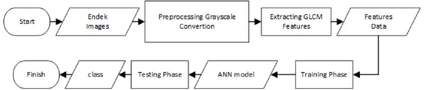
Figure 1. Flowchart System
As seen in figure 1, endek images have to be converted into grayscale format so that images will only have one color channel. Later, system can performes feature extraction using GLCM algorithm to these images. These GLCM features will act as input for the artificial neural networks in the training and testing phase. Output classes from testing phase is endek cloth variances which are endek cloth variances which are cemplong pattern, sekar pattern, gringsing pattern dan wajik pattern.
This research uses Python 3 programming language with GLCM algorithm from the sklearn library and tensorflow framework version 2.0 as the base for programming the artificial neural network. This framework provides a variety of layer object models and optimizers that can be customized according to user requirements.The artificial neural network model which was formed in this research consists of 16 input neurons.
The data used in this study are secondary data types obtained from [2]. This data contains 4 types(later we will use as class) of endek cloth with different patterns, such as endek cemplong, sringsing, sekar dan wajik(diamond). each class contain approximatey 60 images with a resolution of 40 x 40 pixels.. The data will be divided into training data and test data where the training data is 80% of the total data and test data is 20% of the total data.
Artificial Neural Network is one of the artificial representations of the human brain which always tries to simulate the learning process in the human brain.
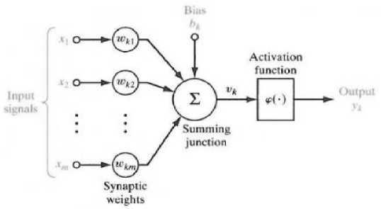
Figure 2. ANN Illustration [2]
Explanation each parts in figure 2:
-
1. A set of synapses, or bridges, each classified by weight or strength.
-
2. An adder to add up the input signals. Weighted from the synaptic strength of each neuron.
-
3. An activation function to limit the output amplitude of the neuron.
The process of forward propagation can be seen in the equations 1, 2 and, 3 [4].
Ztn j = (∑‰1 Xi vlj) + bias(1)
Inputs of each data will be multiplied by the weight and added by the bias of each neuron.
The output of the previous equation will go through an activation function of the neurons.
The output from the hidden layer will go through the activation function of the classification neurons.
Table 1 shows details and the activation functions of each layers of ANN models that had been formed in this research. Number of neurons in the hidden layers are based on rules which are provided from previous research [4].
Table 1. Detail Each Layer
|
Layer |
Number Of Neurons |
Activation Function |
|
Input Layer |
16 |
- |
|
Hidden Layer 1 |
29 |
Relu |
|
Hidden Layer 2 |
8 |
Relu |
|
Classification Layer |
4 |
Softmax |
The learning process of the neural network model uses the epoch variable as the maximum number of learning cycles that the model passes and the learning rate as the weight correction variable in the optimization algorithm. The epochs itself are 1000, 500 and the learning rate is 0.001.
As comparison to Adam's optimization algorithm, this research also used an old optimization algorithm, namely stochastic gradient descent, which is a faster version of gradient descent. Both optimization algorithms use the same epoch values and learning rate. The testing phase is performed twice. First, after model has completed 1 epoch (learning cycle) and secondly testing as final model validation that performed at the end of the training.
Adaptive Moment Estimation(Adam)
Adam an algorithm for first-order gradient-based optimization of stochastic objective functions, based on adaptive estimates of lower-order moments. Adam's algorithm was first introduced in 2015 [3]. The method is straightforward to implement, is computationally efficient,
has little memory requirements, is invariant to diagonal rescaling of the gradients, and is well suited for problems that are large in terms of data and/or parameters.
The method is also appropriate for non-stationary objectives and problems with very noisy and/or sparse gradients [3]. This method is designed to combine the advantages of two recently popular methods: AdaGrad , which works well with scattered gradients, and RMSProp, which works well in setting on-line and non-stationary [3].
Adaptive Gradients (AdaGrad) provides us with a simple approach, for changing the learning rate over time. This is important for adapting to the differences in datasets, since we can get small or large updates, according to how the learning rate is defined [3].
Root Mean Squared Propagation (RMSprop) is very close to Adagrad, except for it does not provide the sum of the gradients, but instead an exponentially decaying average. This decaying average is realized through combining the Momentum algorithm and Adagrad algorithm, with a new term [3].
An important property of RMSprop is that we are not restricted to just the sum of the past gradients, but instead we are more restricted to gradients for the recent time steps. This means that RMSprop changes the learning rate slower than Adagrad, but still reaps the benefits of converging relatively fast [3].
Adam’s weight correction algorithm uses equation 4 5 6 and 7 as follows [5]:
vt = β2 * Vt-1 + (1 - β2) * gt
Vt
1— Pt
υt =
(4)
(5)
(6)
(7)
mt = β1* vt-1 + (1 - β1) * gt2 __ St
t 1 — β1t
mτt
Awt = — η -=---* gt
√V + e
wt+1 = wt + Awt
Where :
η = initial learning rate
gt = gradient at time t (step / epoch) along wt.
vt= the exponential average of the gradient along wt.
st = the exponential average of the squares of the slope gradient along wt.
Where in Adam itself there are 2 hyperparameters that can be adjusted based on the needs of training model. The hyperparameters are β1 and β2. By default each parameter has the following values:
β1 = 0.9
β2 = 0.999
Parameter e is a very small value to avoid zero division [5]. e = 10-8
ReLu
ReLU (Rectified Linear Unit) is one type of activation function that can be used in implementing Neural Networks. The basic principle of ReLU operation is that this function will only convert negative input values to 0 values. Equations and illustrations of this function can be seen in equation 8 and figure 3.
ReLU(x) = (0,x)
(8)
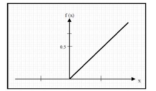
Figure 3. Graphic Illustration of ReLU Activation Function [2]
Softmax
Softmax is an activation function at the classification layer to convert the output vector values into probability values from each label class. If it is known that % is the weighted input received by neurons in the softmax layer, then the activation yj for neuron j-th can be seen in equation 9.
cx^ softmax(yi) = =r77-----—
(9)
∑n=i eχk
It can be said that in the Softmax layer, the output is a probability distribution for each class. The denominator ensures that the ith output is close to 1. Using softmax we can interpret the network output y" as an estimate p(xn).
Cross Entropy Error
The softmax activation function that is applied to the fully connected layer (fc layer) will be paired with cross entropy. This cross entropy will later be used for calculating the amount of loss or error value from the softmax output against the expected output. The cross entropy error can be calculated using equation 10 as follow :
N
Cross enthropy(x^) = -
∑ i=ι
p(Xi) * log(q(xi))
(10)
GLCM is one of the feature extraction methods to obtain feature values by calculating the probability value of the co-ocurrence matrix from the adjacency relationship between two pixels at a certain distance and angular orientation [6].
The direction and distance of the GLCM can be seen in Figure 4. Figure 5 shows the process of calculating the GLCM co-ocurrence matrix [6].
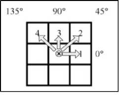
Figure 4. GLCM Angle Illustration [6]
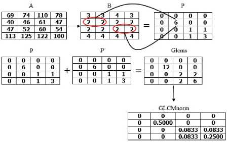
Figure 5. Illustration of calculating co-ocurrence matrix [6]
-
16 inputs of ANN are derived from the four (4) directions adjacency matrix of cooccurrence matrix of GLCM which later for each direction will have four (4) image features extracted using equations 11, 12, 13, and 14. Foreach image, there are number of directions multiple by number of features that become as input, 16 inputs in this case.
The statistical features of GLCM extracted from grayscale images in this research are as follows[6] :
1.
Entropy
Entropy is used to measure the randomness of the intensity distribution [6]. Entropy
Equation [7]:
Ent - -∑m∑∕lp(i,j)log{p(i,j)}
(11)
-
2.
Energy
Energy is a feature of GLCM which is used to measure the concentration of intensity pairs on the GLCM matrix [6], and is defined as follows. Energy Equation [7]:
-
3.
TT- Γ mm p(i,j) "-∑,∑i ι + (i-j2)
(12)
Homogeneity
Shows the homogeneity of the intensity variation in the image [6]. The Homogeneity equation is as follows [7]:
fi = ∑m∑∕lp(i,j)2
(13)
4.
Contras
Contrast is the calculation of the difference in intensity between one pixel and adjacent pixels throughout the image [6]. Zero contrast for a constant image. Contrast Equation as follows [7]:
(14)
C2- ∑m∑=o Paj)(i-J)2
Where [7]:
P = normalized GLCM matrix i = row index matrix P j = column index matrix P
As previously written in research method. We use 4 types(later we will be written as classes) of endek cloth with different patterns, such as endek cemplong, sringsing, sekar dan wajik(diamond). Each class contain approximatey 60 images with a resolution of 40 x 40 pixels.
Before splitting data into 2 categories, we convert these images into grayscale and later on we extract its 4 statistical features from each grayscale version of the image. After we got these features data,The data will be divided into training data and test data where the training data is 80% of the total data and test data is 20% of the total data.
This research will evaluate the neural network model twice, which one is performed after each leaning cycle or epoch later we will include graph to illustrate accuracy and loss for each epoch and second is performed after learning step finished to final test the model which has been formed. These two testing use same data which is 20% of the total data.
As previously written, each optimizer algorithm will be tested by using several epoch and same learning rate that is for epoch are 1000 and 500 and for learning rate is 0.001. Later we will note and compare accuracy and loss value generated by these variables to find which one has the highest accuracy.
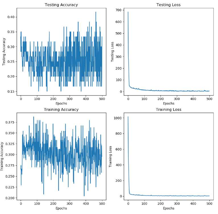
Figure 6. Epoch 500 and 0.001 learning rate
You can see the training and testing accuracy graph in Figure 6. Accuracy in the learning process is in the range of 20% to 37.5%. While at the testing stage, the model accuracy for each epoch is in the range of 15% to 40%. After completing the entire training process and entering the second testing phase for final validation of the model that has been formed. The final model accuracy is 33%.
As seen in the loss value graph, both the training and testing graph in Figure 6, there is a tendency for the loss value to fluctuate but not significantly. This indicates that the Adam optimization algorithm does not experience a situation where it stucks in a local minima when finding the lowest point or minimum loss value which is called the global minima of the objective function.

Figure 7. Epoch 1000 and 0.001 learning rate
You can see the training and testing accuracy graph in figure 7. Accuracy in the learning process is in the range of 23% to 45%. While at the testing stage, the model accuracy for each epoch is in the range of 10% to 53%. After completing the entire training process and entering the second testing phase for final validation of the model that has been formed. The final model accuracy is 28%.
As seen in the loss value graph, both the training and testing graph in Figure 6, there is a tendency for the loss value to fluctuate but not significantly. This indicates that the Adam optimization algorithm does not experience a situation where it stucks in a local minima when finding the lowest point or minimum loss value which is called the global minima of the objective function.
It can be seen in the 4 graphs shown in Figure 8. Accuracy in the learning process at the initial epoch is in the range 19% to 26%, then the accuracy looks quite constant around 25.5% to 26%. While at the testing stage, the accuracy of the model for the initial epoch is in the range of 21%, then it looks constant at 23.25%. After completing the entire training process and entering the second testing phase for final validation of the model that has been formed. We got a final model accuracy of 23%.
As seen from the loss graph in each epoch both at the training and testing stages. SGD has a tendency that changes in the loss values are insignificant (illustration on the testing loss graph) and even flat (illustration on the training loss graph). Of course this can be caused by two possible circumstances, namely, the model has reached the global minima or the model is stuck
in a local minima without, previously reaching the global minima. Look at figure 10 to get an illustration of the local minima and global minima.
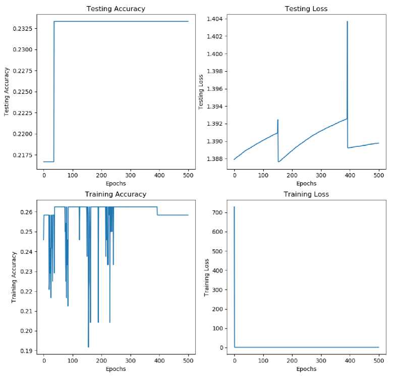
Figure 8. Epoch 500 and 0.001 learning rate
It can be seen in the 4 graphs shown in Figure 9. Accuracy in the learning process at the initial epoch is in the range 20% to 26%, then the accuracy looks quite constant at 26%. While at the testing stage, the accuracy of the model for the initial epoch is as high as 28%, then it looks dropping down and constant at 21.5%. After completing the entire training process and entering the second testing phase for final validation of the model that has been formed. We got a final model accuracy of 21%.
As seen from the loss graph in each epoch both at the training and testing stages. SGD has a tendency that changes in the loss values are insignificant (illustration on the testing loss graph) and even flat (illustration on the training loss graph). Of course this can be caused by two possible circumstances, namely, the model has reached the global minima or the model is stuck in a local minima without, previously reaching the global minima. Look at figure 10 to get an illustration of the local minima and global minima.
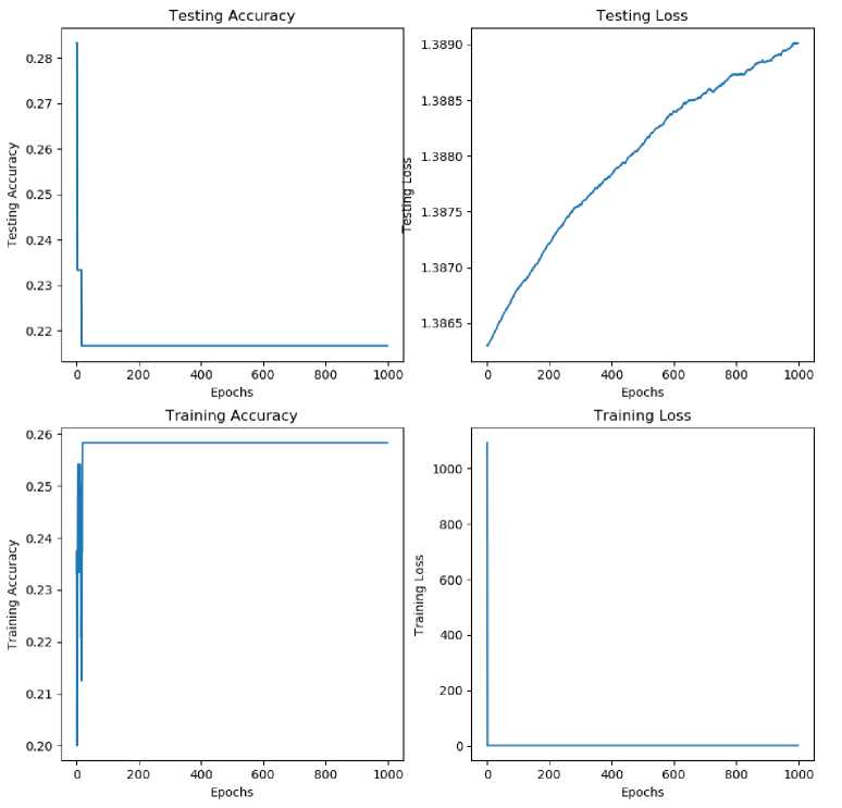
Figure 9. Epoch 1000 and 0.001 learning rate
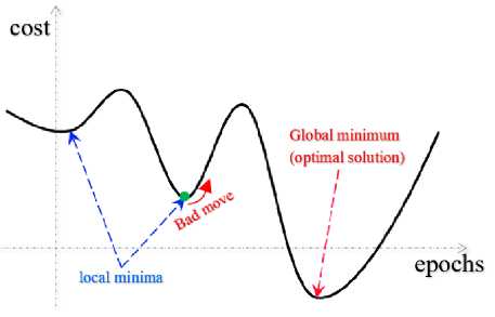
Figure 10. Ilustration of Local Minima and Global Minima
In Figures 7 and 8, it can be seen that Adam's algorithm has a tendency to change the loss value up and down but not so significant. This is due to the advantages of Adam itself which can move from each local minima without experiencing any stuck or trap conditions. In accordance with the advantages of the Adam algorithm as previously written, this advantage is obtained from the elements of the Adagrad algorithm which are arranged in the Adam algorithm.
In Figures 9 and 10, it can be seen that the SGD algorithm, unlike Adam's algorithm, has a tendency to change the loss value which is thin and insignificant. This is due to the possibility
that the model is stuck on a local minima with a poor level of accuracy. This situation causes almost constant accuracy at the training and testing stages of the SGD.
Final accuracy result of each algorithm with different epochs are given in table 2.
Table 2. Model Accuracy
|
Number of Epoch |
Stochastic Gradient Descent Learning Rate 0.001 |
Adam (Adaptive Moment Estimation) Learning Rate 0.001 |
|
1000 |
21 % |
28 % |
|
500 |
23 % |
33 % |
Shorter epoch also generates better model performance for both optimizer algorithm. Adam algorithm generates higher accuracy than the accuracy that is generated by the algorithm SGD. This can be proven from the training accuracy graph, the first testing phase accuracy graph and the final accuracy of the model. The poor SGD accuracy results from being stuck in a local minima with low accuracy. Meanwhile, Adam's better accuracy is indirectly related to the nature of the algorithm itself which does not experience the problem of being trapped or stuck in cases with scattered gradients.
Other thing that get our concern is both SGD and Adam algorithm give terrible accuracy. So that we use another classification algorithm to classify and evaluate our training and testing data. We used KNN classification algorithm to test our data. Unlike artificial neural network, KNN give a little bit better accuracy which is 45%. But still, both classification algorithm give accuracy which is below 50%. This result can be categorized as poor performance. We can conclude that GLCM has difficulty to generates good feature data for classification of endek cloth case.
This terrible performance can be occurred because of each variance of endek cloth has almost similar GLCM texture value when compare to the others. Unlike GLCM, deep learning can extract or detect edge inside any images. As proven in previous research CNN which gave 80% average accuracy. This edge cannot be detected using GLCM. Edges is a strong feature when classify images cases based on pattern. As written above, endek variances are differentiated using pattern.
Based on accuracies of each model which had been formed. Using 500 as number of epoch or training cyclies, generates better model performance for both optimizer algorithm. Adam optimization algorithm performs better than SGD optimization algorithm in this classification case. As given accuracies from graph figures and both final testing phase, SGD algorithm gives 23% and Adam algorithm gives 33%. Secondly, the GLCM feature extraction method used to extract features from the endek images gives poor result of features data when used for classification. This can be seen from the accuracy of the models from two algorithms are below 50%. This poor performance can be occurred because, one, each variance of endek cloth has almost similar GLCM texture value when compared to the others. Secondly, GLCM cannot detect edge feature which is a strong feature in pattern based image classification. Based on these results, we strongly advice for the next research to use extraction algorithm based on edge detection or use one of deep learning architecture and utilize advance optimizer algorithm to achieve better performance.
References
-
[1] I. G. S. Rahayuda, “Texture Analysis on Image Motif of Endek Bali using K-Nearest Neighbor Classification Method”, (IJACSA) International Journal of Advanced Computer Science and Applications, vol. 6, no. 9, 205-211, 2015.
-
[2] I. K. R. Dewantara, “Implementasi Deep Learning Menggunakan Convolutional Neural Network (CNN) Untuk Identifikasi Jenis Kain Endek Bali”, Skripsi Jurusan Ilmu Komputer Fakultas Matematika dan Ilmu Pengetahuan Alam. Bukit Jimbaran, pp., pp., 2019.
-
[3] D. P. Kingma and J. Lei Ba, "ADAM: A METHOD FOR STOCHASTIC
OPTIMIZATION", Published as a conference paper at ICLR 2015, pp, pp. 1-15, 2015.
-
[4] M. S. Wibawa, “Pengaruh Fungsi Aktivasi, Optimisasi dan Jumlah Epoch Terhadap Performa Jaringan Saraf Tiruan,” JURNAL SISTEM DAN INFORMATIKA , Vol. 11, No. 1, 1-8, 2016.
-
[5] S Bock, J. Goppold and M. Wei, . “An improvement of the convergence proof of the ADAM-Optimizer”, Conference Paper At OTH Cluster Konferenz, pp. pp. 2018.
-
[6] N. Zulpe and V. Pawar, "GLCM Textural Features for Brain Tumor Classification", IJCSI International Journal of Computer Science Issues, vol. 9, no. 3, pp. 354-359, 2012.
-
[7] http://www.mathworks.com/help/images/gray-level-co-occurrencematrix-glcm.html. Diunduh 15 Agustus 2020.
296
Discussion and feedback