Growth, Inequality, and Poverty: An Analysis of Pro-Poor Growth in Indonesia

Written by Yudistira Andi Permadi
on August 13, 2018

JEKT ♦ 11 [2] : 216-233

pISSN : 2301 - 8968 eISSN : 2303 - 0186

Yudistira Andi Permadi

ABSTRACT

In the concept of pro-poor growth, economic growth accompanied by fair income distribution will accelerate the rate of poverty reduction. By employing extensive data of household expenditures and other economic indicators, the study will examine the performance of economic growth in Indonesia whether it has been pro-poor over the period 2005-2013. We employ two methods in this article, Growth Incidence Curve (GIC) method, and Pro-Poor Growth Index (PPGI) method. By applying the GIC method, our empirical results indicate that economic growth in Indonesia has not been pro-poor during the observed period. The curve shows that the highest income population enjoys increased consumption more than the poorest population. Furthermore, PPGI method has revealed that economic growth, inequality, and an interaction term between economic growth and inequality have been significant to influence poverty incidence in Indonesia. Our empirical result also reveals that among manufacturing, agriculture, and services sector; it was manufacturing that has successfully reduced the number of the poor, while agriculture unexpectedly had a devastating impact on the number of poor people. The services sector, meanwhile, had not contributed to poverty alleviation. Furthermore, none of the government spending in education and health that significantly contributes to poverty alleviation.

Keywords: Poverty, Economic Growth, Inequality, Pro-Poor Growth

Pertumbuhan Ekonomi, Ketimpangan, dan Kemiskinan: Sebuah Analisis Pro-Poor Growth di Indonesia

ABSTRAK

Dalam konsep pertumbuhan ekonomi yang pro-poor, pertumbuhan yang disertai dengan pemerataan pendapatan akan mempercepat proses pengentasan kemiskinan. Dengan menggunakan data survey pengeluaran rumah tangga dan berbagai indikator ekonomi, penelitian ini akan menguji apakah pertumbuhan ekonomi Indonesia pada periode 2005 sampai dengan 2013 dapat dikategorikan sebagai pertumbuhan yang pro-poor. Penelitian akan menggunakan dua metode, yakni metode Growth Incidence Curve (GIC) dan metode Pro-Poor Growth Index (PPGI). Metode GIC menunjukkan hasil empiris bahwa pertumbuhan ekonomi pada periode yang diobservasi tidak bisa dikatakan sebagai pertumbuhan ekonomi yang pro-poor. Kurva GIC memperlihatkan bahwa rumah tangga ‘kaya’ justru menikmati peningkatan pengeluaran untuk konsumsi dibanding rumah tangga ‘miskin’. Lebih jauh lagi, ketika menggunakan metode PPGI, dapat disimpulkan bahwa pertumbuhan ekonomi, ketimpangan, dan interaksi antara pertumbuhan ekonomi dan ketimpangan berpengaruh secara signifikan terhadap kemiskinan di Indonesia. Hasil empiris juga menunjukkan bahwa dari tiga sektor yang diteliti, yakni sektor industri, sektor pertanian, dan sektor jasa; sektor industri berpengaruh positif dan signifikan terhadap upaya pengentasan kemiskinan, sedangkan sektor pertanian justru secara signifikan berkorelasi negatif dengan pengurangan kemiskinan. Sementara itu, sektor jasa tidak terbukti berkontribusi dalam menurunkan angka kemiskinan. Selain itu, uji statistik juga menyatakan bahwa pengeluaran pemerintah di bidang pendidikan dan kesehatan tidak berkontribusi dalam mengurangi kemiskinan.

Kata Kunci: Kemiskinan, Pertumbuhan Ekonomi, Ketimpangan, Pro-Poor Growth

1. Introduction
- 1.1. Background

Poverty reduction is one of the most important goals in economic development. In the development perspective, poverty is an obstacle that blocks human beings to meet their basic needs. It could also pull the trigger of many social problems within society, such as crime, poor health, or mental illness. Given the enormous negative impact in social life, efforts to alleviate poverty, therefore, should be prioritized in the development agenda.

In the development program, economic growth is believed to be the best potion to cure poverty. The importance of economic growth was initially emphasized by a concept, famous in the period of 1950s and 1960s, called a trickle-down hypothesis. The main idea of the theory believes that growth alone can reduce the number of poor people. The concept states that the benefits of growth will come first to rich people, and eventually, the benefits will stream down to poor individuals in the society. It is said that “the poor can only have benefited indirectly through a vertical flow from the rich; thus, the proportional gain from the growth will always going less for the people” (as cited in Kakwani and Pernia 2000: 2).

The best example of the essential role of economic growth on poverty alleviation is shown by the story of the People’s Republic of China (PRC). Based on the World Bank database, PRC is now recognized as one of the world’s economic giants regarding per capita income. The country has been able to achieve their success since the government promoted economic reforms, started in the 1970s, with the focus on high economic productivity. The effort has shifted the country from ninth to the second position in Gross Domestic Product (GDP) globally. Studies by Lin (2003) and Montalvo and Ravallion (2010) confirmed that economic growth in PRC has successfully reduced poverty in China. However, regarding income distribution, PRC is also known for a high degree of inequality. Before the economic reform, PRC was acknowledged as an egalitarian society. By 2012, World Bank (2017) published that the Gini ratio in PRC is recorded at 42.2%.

While PRC’s evidence shows us the magnificent effect of growth on poverty; however, some economists have their doubts over the validity of the argument that poverty reduction solely

depends on economic growth. One of the concerns over trickle-down concept is that in some cases, there are possibilities that increasing poverty rate could also accompany high economic growth. Past experiences have revealed that it was the rich who got more advantages or welfare from the economic growth thus, the gap between the poor and the rich became larger. Bhagwati (1988) called this situation as “immiserizing” growth, a situation where inequality has a greater impact than the benefits of economic growth. Therefore, – it creates deterioration by increasing the number of poor people (as cited in Kakwani and Pernia 2000: 2).

As a consequence, there is argument suggesting that the poverty alleviation program will be useful when growth is accompanied by the even distribution of income (Kakwani and Son 2003; Kakwani et al. 2010). This argument believes that not only the income growth is necessary for poverty alleviation, but also the quality of income distribution. When economic growth is followed by equal distribution of individual income, the poor will likely have better chance to obtain more income. So, people who are below the poverty line can improve their welfares and escape poverty.

The debate over the measure of pro-poor growth, therefore, can be sum up into two different perspectives. The first is the argument which does not explicitly emphasize the need for inequality when measuring pro-poor growth. This case believes that the only matter when determining pro-poor growth is the change of poverty level within the observed period, while the change in inequality is naturally only a part to achieve poverty reduction (Ravallion and Chen 2003; Ravallion 2004). According to the proponents, pro-poor growth is an increase of national income accompanied by a decrease of the poverty level. In other words, as long as the decline in poverty follows economic growth, we can still categorize it into pro-poor growth, despite no improvement in the distribution of the income. However, they believe that if the benefits are well distributed within the society, economic growth will produce the higher magnitude of poverty reduction.

The second is the argument which takes into account inequality when measuring pro-poor growth. This view believes that growth is propoor when the poor not only achieve gain from economic to meet the basic necessities but also

receive more benefits of growth than those who are not poor (Kakwani and Pernia 2000; Kakwani and Son 2010). According to these proponents, propoor growth will be achieved when the equitable distribution of income follows growth in total revenues.

The connection between economic growth and inequality on poverty has become an important part in the course of Indonesia’s economic development. Although Indonesia has not experienced fast growth like PRC, Indonesia has tried to establish some strategies to achieve sustainable economic growth. Since the 1960s, those strategies were implemented to reduce poverty level influenced by the concept of trickle-down effect. History proved that the expected result of the trickle-down effect could not be said as the successful one. It was only since 2004 that Indonesia began to formulate the framework outlined in Indonesia’s National Medium Term Development Plan to implement the three strategies of economic development, which are a ‘pro-growth, pro-job, and pro-poor’ strategy, while also maintaining equitable income distribution. These three strategies are expected to drive the acceleration of economic growth that can provide more employment opportunities. Thus, more and more people, especially the poor, can enjoy the results of development and get out of poverty.

This study, therefore, is aimed to assess whether or not Indonesia’s economic growth is already propoor. Furthermore, the research also investigates to what extent the impact of economic growth and inequality on the success of poverty alleviation program. The empirical findings of this article are supposed to provide an overview of the success of economic development programs designed in the National Medium Term Development Plan to achieve economic growth that gives benefits more to the poor, in particular through the strategies of pro-poor and pro-growth. Looking at other variables that consist of sectoral composition and government expenditures, the study wants to give added value by revealing which variables have effectively reduced poverty in Indonesia.

1.2. Literature Review
- 1.2.1. Economic Growth and Poverty

It has become the consensus among the economist that economic growth is the minimum requirement

to ensure that poverty alleviation program can be successfully achieved. Son (2007: 3) wrote that to reduce the poverty rate, growth is a minimum recipe but not sufficient to achieve the goal. The reasons are because economic growth can generate income effect and help the poor to raise their revenues, create job opportunities, and generate multiplier effects resulting from increased income (Nayyar, 2005). Todaro and Smith (2009) have even stressed the need for poverty alleviation program and economic growth to be achieved mutually.

The relationship between economic growth and poverty reduction has been supported by numerous findings that attest the beneficial effect of economic growth to the poor (Wodon 1999, Dollar and Kraay 2002, Bourguignon 2004, Warr 2006, Perera and Lee 2013, Dollar et al. 2016). Nevertheless, the success of economic growth to reduce poverty is believed to be highly correlated with the characteristic of each country like initial income, the human capital level, or institutional quality (Pernia 2003: 1).

1.2.2. Inequality and Poverty

Kakwani and Son (2003: 417) stated that the policy to reduce the poverty level need to be considered the better distribution of income so that the poor people will gain more in the development agenda. It is the rich who usually obtain a large sum of income when a country experiences economic growth. So, if poverty reduction is reached through the equitable distribution of income, then all components of the economy can contribute to accelerating economic growth (Bourguignon, 2004). Bourguignon (2004), however, stated that the effects of economic growth and inequality on poverty might differ from one country to another depending on the initial level of income and inequality. In other words, when a country wants to implement a policy to reduce poverty level during a particular time, the state should consider the initial condition, like income level or inequality. Nonetheless, Simon Kuznets (1955), claimed that there is also an exclusive bond between economic growth and inequality that could result in a trade-off between inequality and poverty. He revealed that in the early stages of economic growth, income per capita would increase at a certain level and is accompanied by rising inequality level. At this period, poverty falls but inequality rises, and therefore, the trade-off

happens.

Some empirical studies have proved that the improvement in income distribution could bring a greater chance of poverty reduction (Ravallion and Chen 1997, Wodon 1999, Lin 2003). They were all agree that the increase in inequality reduced the effectiveness of economic growth. Lin (2003) also put a notion that the initial level of inequality is essential to determine growth policy within countries with different stages of development. Ravallion and Chen (1997), meanwhile, believed that the effect of inequality on poverty has not been strong enough to reduce the elasticity of growth in poverty. By employing cross countries data obtained from the household surveys of sixtyseven countries, they come to conclusion that in developing countries, the impact of inequality on poverty was not statistically significant. It means that if developing countries could not raise their income level, the rate of poverty reduction was expected to be zero. A different argument was proposed by Ravallion (2005) who found a tradeoff between absolute inequality, as reflected by absolute Gini index and poverty. This means that increase in absolute inequality still possibly reduce the poverty level. However, when it turned to relative inequality, such of trade-off did not happen.

1.2.3. Economic Growth, Inequality and Poverty

Many studies, such as Silva (2016) and Maasoumi and Mahmoudi (2013) have been conducted to investigate the relationship between economic growth, inequality, and poverty. Silva (2016) decomposed the changes in poverty level into two components, economic growth and inequality, one of which is based on GIC proposed by Kakwani and Pernia (2000). Using GIC, the study concluded that only the top percentile of the population in Sri Lanka increased spending more than average growth rate of expenditures. This means “just a few households moved up along with the average growth rate of the economy” (Ibid.). The impact of redistribution component had a positive sign, meaning that an increase in inequality would raise poverty. Meanwhile, the negative sign of the effect growth on poverty implies that increased growth will reduce poverty. Therefore, the positive impact of economic growth in poverty level was reduced by the effect of inequality on poverty. Similarly, Maasoumi and Mahmoudi (2013) in their article

supported the idea of the good effects of economic growth on poverty reduction and the adverse effects of inequality on poverty level.

Methodology

2.1 . GIC Model

The study utilises the model developed by Ravallion and Chen (2003: 95) and Ravallion (2005: 21) which can be represented as follow:

g(p)=γ+dLn(L^,(p))

γ : dLn(μ) that is the growth rate of mean consumption expenditure

L’(p) : first derivative of Lorenz function

g(p) : GIC

This method analyses the movement of the growth of mean consumption per capita across the p-percentile of the population, and then we make a conclusion whether the poor have received more benefits than non-poor in the economy. The process to measure GIC is as follow:

a. Calculating the mean consumption per capita of the population obtained from the National SocioEconomic Survey in 2005 and 2013 which cover all of regencies and municipalities in Indonesia.
b. Adjusting data to be comparable to time and region.
c. Sorting the percentile distributions of expenditures from the lowest percentile to the highest percentile in each year.
d. Calculating the growth of mean consumption per capita for each percentile by using geometric growth formula:

_r=M^v"-ι

where r = growth, p_2005 = mean consumption per capita year 2005, p_2013 = mean consumption per capita year 2013, and n = 8 (2013 – 2005 = 8) e. Calculating mean growth using software Microsoft Excel.

This method is analyzing the shape of a curve generated from the change in income or expenditure level between two periods of time, then concluding whether or not growth is already pro-poor. The vertical axis of the curve represents growth in revenue or expenditure level, while the horizontal axis represents percentile of the

population. As a basis to determine whether each percentile has already enjoyed benefits of growth, the curve is equipped with a line which represents the mean of consumption expenditures or incomes among the population. If the curve intersects the line of mean income or mean expenditure from the top left to the bottom (downward sloping), it can be concluded that economic growth is pro-poor and vice versa, if not (upward sloping) then not pro-poor.

GIC method has an advantage since it can indicate changes in income inequality between the poor and non-poor. If GIC is a downward sloping, it means that income inequality also decreases. Conversely, if GIC is an upward sloping, the distribution of income is getting worse. Aside from its advantage, if the curve does not take the shape of either downward sloping or upward sloping, then we could not conclusively determine whether or not growth is already pro-poor.

2.2 PPGI Model

In this method, the study refers to the model proposed by Wodon (1999) which has calculated the impact of economic growth and inequality to poverty in Bangladesh. However, this study modifies the basic model by adding some determinants which theoretically and empirically can affect poverty; so that, the results provide a better understanding of the performance in poverty reduction during observed periods.

The model can be described as follow:

P0_it=ω+γlogY_it+δG_it+θ(logY_it*G_it)+ϕ₁logeducation+ϕ₂loghealth+Ω₁agriculture+Ω₂manufacturing+Ω₃ service+ ω_i+ε_it

P0 : Headcount Index (the

percentage of poor people)

Y : GRDP per capita at constant

price 2000

G : Gini ratio

education : the amount of government

spending in education

health : the amount of public

spending in health

agriculture : the ratio of output in

the agriculture sector to GRDP of regency or municipality

manufacturing: the ratio of production in

the manufacturing sector to GRDP of regency or municipality

service : the rate of output in the

service sector to GRDP of regency or municipality ω : intercept (fixed/random

effect for district-i)

ε : error term

i : cross section – regencies/

municipalities

t : time – t

In the model, γ is a parameter of the log of

GRDP per capita, δ is a parameter of Gini ratio, and θ is a parameter of the interaction between the log of GRDP per capita and Gini ratio. By using interaction variables, the effect of economic growth or inequality on poverty also depends on the interaction between the two. Furthermore, the parameters of ϕ and Ω represent how the changes of other explanatory variables could affect poverty incidence. Furthermore, ϕ₁ represents the parameter of the log of education spending, ϕ₂ represents the parameter of the log of health spending, while Ω₁, Ω₂, and Ω₃ represent the parameter of sector shares in agriculture, manufacturing, and services to GRDP respectively. The sign of those parameters can be either positive or negative depends on their influence on poverty. When the sign is positive, then the variable has a positive link to poverty incidence. However, when the parameter sign is negative, the variable has been a success in influencing poverty reduction.

To see how all variables on the right side of the model have affected poverty, we analyze the best model meant for panel data set, namely common effects, fixed effects, and random effects model. Nonetheless, since the study refers to the work by Wodon (1999) which used fixed and random effects in his estimation, the study; therefore, selects which one between fixed and random effects that is best to answer the research question. The Hausman specification test is then performed to choose between fixed and random effect. However, the selection of the best panel data model between fixed effect and random effect can also be made with non-statistical considerations. Non-statistical consideration used here is by comparing the number of individual or cross section unit and time series unit. It is said that when panel data set has time series unit less than cross section unit;

Table 1 Data Sources

Mci	Vnriiabls	I ^,πoxy	HoriLrt	Puhhiihsr
	I¹CvrtlA-	11 s-.il Iron r I Jriclrtjt	DjIh Hricl ]rιToirnHLiun ol Porrcrty 2005-2 C¹L ?	SLiLiiiLiL Erickirirtiiij
Z.	I iLcκιorιiι Cioivtji	CiKIJ]^1, fIrti CiipiLi	CiI-LDP ol I-Irts;s-ι√im; jruJ MiinicrMiLitics .d Ie: ODOijf 2005-20L3	SLlLillLlL ilhkl'lrt-.ij
	[rise ILiiJiIy	Ciini rj∣ιo	MjIioilhI Sul ic: Lroiioiiiie Siirvcy 20Φ5-20 J 3	SLiLriLiL 11 h k∣' ∣rt-.r a
■1.	Cii R-S-I i ιιns'i. Spflldjng	I J-IlJLJllCji: HIXl .Irtilllll Spo-Jjdjixg	AiiiliisJ l-Lspij∣∣ of RcgCDfjCS fJLC MLlLLjcipflLitjcs .D IEC Onfijf ^,tκ∣5 znn	DinKjLLirdLei Catfiirtml o: Fiscal Balfjjcc -MirJiiLy ofFinancc
	Sectoral LcizripLiiiilioi:	ApLjcilLtllTC, n∣j∏u Γjl Luri up.. hii∣I Iierc ic s:; ikl Ic: i	GRPP of RjCCCLiCLCi and Murιiciτxali Liιa-, in IniJnnBcciii ^,(lil.ι ZO ∏	Statjarif IDdoucaia
6.	C OJlSllJUOtjon psr L HfiJii	Ilor-EllJLVljOD p?L LiipiLa	NacioED] Socic-Zcojionijc Si Iivrty ∩j∣ Lirtyrtiii ZCKL^	Statiarif Indonesia

ιιnιJ ¹CI i

then random effect model is better. However, when time series unit is more than cross section unit, then fixed effect model is better (Baltagi 1994, Nachrowi and Usman 2006)

3. Data

All the variables which become the focus of the research are economic growth, proxied by Gross Regional Domestic Product per capita at constant market price 2000, inequality proxied by Gini ratio, and poverty proxied by Headcount Index or P0. The study uses an interaction variable between economic growth and inequality in explaining how these two variables affect poverty. Moreover, some control variables used in the model are government spending in education and health and sectoral composition which consists of three sectors in the economy, agriculture, manufacturing, and services. All the data are the secondary source at the regional level (regency and municipality) in Indonesia obtained from various reports of Indonesian Statistic and Directorate General of Fiscal Balance for the period of 2005-2013. Meanwhile, the data used for estimating Growth Incidence Curve is calculated from per capita expenditure based on the National Socio-Economic Survey in 2005 and 2013 published by Indonesian Statistics. The summary of data used in this study is presented in Table 1.

Poverty

The proxy of poverty in the model is Headcount Index, published by Indonesian Statistic, based

on data from National Socio-Economic Survey. The method to measure poverty line is called the Cost of Basic Need Method, a method that requires “households to meet their basic needs of food and essential non-food spending” (World Bank 2005: 54). The class of poverty measures is estimated by the method proposed by Foster, Greer, and Thorbecke (1984):

«r

^p"' ⁼ ⅛ Σ ^max ^^{1 -} Σ^,2'⁰^

“y_it is consumption expenditure of the i’th person at date t in a population of size N_t, z is the poverty line, and α is a non-negative parameter” (as cited in Ravallion and Datt 2009: 6). When α=0, α=1, α=2 the measures are called the Headcount Index, the Poverty Gap, and the Poverty Gap Index respectively.

3.2. Economic Growth

Ravallion (2004) said that household incomes and expenditures or Gross Domestic Products could be used as a proxy for economic growth. This study uses GRDP per capita to find the effect of economic growth on poverty.

3.3. Inequality

The measure of inequality in the model uses Gini ratio issued by Indonesian Statistic.

3.4. Interaction Variable between Economic Growth and Inequality

Table 2 Descriptive Statistics

Variable	Ofes	Mean	Std. Dev.	Min	Max
PO	4.239	16.212	9.75	1.33	54.950
grdppercap	4.452	8,182.486	12,500.000	387,474	217,000,000
gi∏i	4,238	0.295	0.054	0.072	0.566
agriculture	4.454	0.328	0.192	0.0002	0.942
manufacturing	4.454	0.122	0.145	0	0.942
sendees	4.454	0.127	0.073	0.0029	0.482
health	3,320	70,100.000.000	76,000,000.000	1.050.000.000	1,950,000,000.000
education	3,312	219.000,000.000	239,000,000.000	101,000.000	5,550,000.000,000
g∏bLiaisi	4,238	4.596	0.920	1.033	9.702

The interaction variable between growth and inequality in the model refers to study by Bourguignon (2004). He stated that the relationship between economic growth and inequality to poverty reduction is not merely like two separate arithmetic relationships. Instead, the interaction between economic growth and inequality does exist and influences poverty alleviation. His argument is based on some findings in microeconomic-based research which indicates the correlation between economic growths on income distribution (Ibid.).

3.5. Government Spending in Education and Health

Government expenditures on education and health in the model is the total amount of payment specifically allocated to finance various activities in education and health. The activities include operational costs, wages for staff, and transfer for social protection.

3.6. Sectoral Composition

Sectoral composition in the study shows the percentage contribution of each sector in producing goods and services to national account. Sectors used in the model include the agriculture sector, manufacturing sector, and service sector.

3.7. Descriptive Statistic

Table 2 summarizes the statistical description of all variables in the study.

We can see from table 2 that the gap between the lowest and the highest of some variables like GRDP per capita and government spending on health and education is quite enormous. The difference can be

easily understood by giving the size of the economy between the ‘established’ and ‘underdeveloped’ regencies or municipalities in Indonesia. What is needed to be noticed here is that there were some regencies with no contribution of manufacturing sector to the total output regionally. Those regions mostly depended on agriculture sector as their primary sector in the economic activities.

4. Empirical Results
- 4.1. GIC Model: Pro-Poor Growth

GIC is used to determine the extent to which economic growth has provided benefits to the poor. The economic growth can be called as propoor when GIC shows downward sloping from the lowest percentile to the highest percentile. It means that the poorest have increased their income or expenditures more than the richest population. Meanwhile, growth in the economy is not pro-poor if GIC shows upward sloping or the growth rates increase monotonically from the lowest percentile to the highest percentile. In other words, those who are in the highest percentile receive more benefits of growth than the people at the lowest percentile. However, when the curve does not take the shape of either upward or downward slope, we cannot indicate whether growth is pro-poor or not.

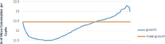
This study, meanwhile, has divided population into 100-percentile which reflects the distribution of expenditures by different households ranked to their consumption level. From 2005 to 2013, according to Figure 1, growth in mean consumption per capita was positive for all percentiles, indicating that the entire population had experienced increasing expenditures. From the GIC, it also can

Figure 1 Growth Incidence Curve

Indonesia: GIC 2005-2013

f ¹¹S ^w 10.5

1 5 9 13 17 21 25 29 33 37 41 45 49 53 57 61 65 69 73 77 81 85 89 93 97

Source: STATA Computation and Microsoft Excel 2013

be concluded that “there is first order dominance, which implies that poverty has fallen no matter where one draws the poverty line or what poverty measure one uses within a broad class” (Silva 2016: 1286).

However, it can be seen that the bottom 20% percentile only experienced an increase in consumption with a value less than the mean growth, while the top 20% percentile enjoyed increases in consumption more than the average growth of consumption expenditures. In general, the slope of curve implies rising inequality over the period of 2005-2013 since the households in the top consumption percentile had a higher growth rate of consumption than the poor. Because the poorest still only experienced lower growth rates of consumption than the average growth of consumption, we could not claim that economic growth of Indonesia was already pro-poor during the observed periods.

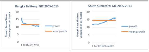
While at the national level, Indonesia’s growth cannot be called as pro-poor growth, we can observe that at the provincial level, some of the provinces have already achieved a pro-poor growth. Based on Figure 2, the GIC curve of Province of Bangka Belitung for example, shows a negative slope where the bottom 20 % percentile enjoyed an increase in consumption about 15%, whereas the top 20% percentile experienced only 10% growth of consumption. It means that the large share of benefits brought by the growth went to the poor. Meanwhile, the richest still got the benefits, but in smaller proportion. That is what we expect from pro-poor growth, a growth which favors the poor.

On the contrary, in the case of the province of South Sumatera, it was the top 20% who earns huge share of benefits than the bottom 20 %. From the graph, we can see that the poorest only experienced 12% rise in consumption between 2005 and 2013, compared to the richest who enjoyed 16% increase in consumption.

Figure 2 GIC: Bangka Belitung and South Sumatera

Source: STATA Computation and Microsoft Excel 2013

To sum up, the charts above offer two different stories. The first story is a period when growth is favorable to the poor. The second story shows the opposite; it is the rich who take enormous share benefits of growth. From Figure 2, we can say that growth in Bangka Belitung is already pro-poor, but in the case of South Sumatera is not pro-poor. The study has calculated GIC from other provinces as well and finds that among thirty-three provinces in Indonesia, seven of them can be considered have achieved pro-poor growth, while twenty-three provinces are not pro-poor yet. Summary of the results is presented in Table 3 (all results of GIC method at the province level will be shown in Appendix 1).

Table 3 Provinces based on GIC

Type of Provinces (code)

Growth

1. Pro-Poor

3. Cannot be classified

North Sumatera (12), Kepul⅞pan Bangka Belitung (19), Kepulauan Riau (21), East Nusa Tenggara (53), East Kalimantan (64), North Maluku (82), Papua (94)

NAD¹ (11), Riau (14), Jambi (15), South Suniatera (16), Bengkulu (17), DKI Jakarta (31), West Java (32), Central Java (33), Jogjakarta (34), East Java (35), Bali (51), West Nusa Tenggara (52), West Kalimantan (61), Central Kalimantan (62), South Kalimantan (63), North Sulawesi (71), Central Sulawesi (72), South Sulawesi (73), Southeast Sulawesi (74), Gorontalo (75), West Sulawesi¹ (76), Maluku (81), West Papua¹ (91)

West Sumatera (13), Lampung (18), Banfen (36)

Source: Stata Computation and Microsoft Excel 2013

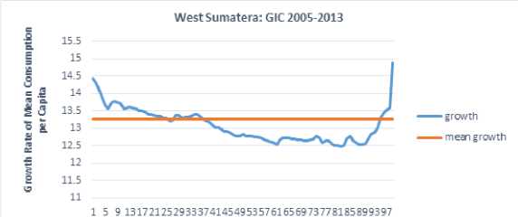
A weakness found in the method is that, sometimes, we encounter a graph which cannot be decided as a curve of pro-poor growth or a curve of anti-poor growth. In Indonesia, three provinces cannot be classified whether they have achieved pro-poor growth or not. They are West Sumatra,

Figure 3 GIC: cannot be classified

Source: STATA Computation and Microsoft Excel 2013

Table 4 The Estimation Result: Random Effects Model

Independent Variables	Poverty (1)	Poverty (2)	Poverty (3)
constant	3111	60.4?	59.12
Grdp	4.10' ^,	-2.86’ "	-2 " "
Gini	(0.61) -13^.1^	(0-63) -134.94"	(O-Sl) -116.46"
grdp -=™	(24.20) 8.'2"	(-3.75) 3.6?"	(28.14) 7.58”'
Agriculture Manufacturing Sendees education Health R overall	(1-53) 0.1 S	(1-52) 13.51" (3-15) -7.77 (5-25) -1.56 (4-2<) 0.23	(1-80) 15.16" (2-94) -9.90' ‘ (4-54) -0.14 (4-52) -0.02 (0.04) -0.01 (0.09) 0.23
(within, between)	(0.5S_z 0.09)	(0.60_i 0.19)	(0.60_z 0.18)
Municipal Regencies	497	490	490
N	4_z235	4_z235	3_z286

Robust Stzndard errors of CoerEerent in parentheses

*, **, *** correspond to a 10,5. and 1% level of significance. Time dummies included in all specifications.

Lampung, and Banten. The example in Figure 3 below shows that the poorest received high shares of growth as well as the richest.

4.2. PPGI Model: The Links between Poverty, Economic Growth, Inequality, the Interaction Term, Government Spending, and Sectoral Composition
- 4.2.1 . Model Specification Test

As described earlier, the study will analyze panel data model. For selecting the best model between fixed effects and random effects, the study then undertakes the Hausman specification test. The result shows that the p-value is 0.000. Therefore, we accept the null hypothesis or the fixed effects is a favor to explain the model.

However, if we take a look at the structure of the data set, it consists of 490 individuals (regencies and municipalities) and 9 years of period (2005-2013). Based on the non-statistical consideration, when the panel data set has individuals number more than time periods, we can choose random effects

model rather than fixed effects model (Baltagi 1994, Nachrowi and Usman 2006). Random effects model basically offers several benefits over fixed effects model (Papyrakis, 2012: 126). The first benefit is it can be used to estimate the impacts of time-invariant variables, which are frequently significant predictors. The second advantage is random effects have more efficient estimators when “combining both the ‘within’ and ‘within’ variation across observations” (Ibid.). Based on those considerations, the study uses random effects specification to analyze the model.

The study will engage some variables other than economic growth and inequality to find which variables have contributed to reduce the poverty incidence during 2005-2013. By employing those variables, the changes in poverty incidence can be better estimated, therefore, we can find the best possible action to ensure the poverty reduction can be achieved effectively.

Table 4 above exhibits the empirical results of random effects specification model. The results

Table 5 The Comparison of Estimation Result: RE and FE

Independent Variables	Random Effects Povert,' (4)	Fixed Effects Poverty (5)
Constant	59.12	47.15
Grdp	-2.7S'"	-1.99
Girii	(0-81) -115.46 ”	(0.80) -118.00'"
gldp_gmi	(28.14) 7.58”	(27.1?) 7.68”
Agriculture	(1-80) 15.16’”	(l-∙4) 12.59"'
Manufacturing	(2-94) -9.90'	(3-90) -12.35”
Services	(4-54) 0.14	(5-29) -7.54
education	(4-52) -0.02	(5-71} 0.01
Health	(0.04) -0.01	(0.04) -0.00
R overall	(0.09) 0.23	(0.09) 0.18
(within, between)	(0.6O_: 0.18)	(0.60, 0.12)
Municipal Regencies	490	490
K	3,286	3,286
Robust standard errors of coefficient m parentheses , _j ** CoiTespcndto a 10,5. and 1% level of significance. Time dummies included in all

specifications

reveal that economic growth, inequality, interaction variable between growth and inequality, agriculture sector, and manufacturing share are strongly linked to poverty incidence in Indonesia. Based on the estimated result, the effects of economic growth and inequality on poverty depend on the interaction variable, while agriculture sector is associated with increasing poverty. However, manufacturing is related with the decline in poverty level. None of the variables consisting of services sector and government spending on education and health have contributed to reducing the number of poor people in Indonesia.

Moreover, when we investigate the model using fixed effects specification, the estimated results are not so much different than using random effects model. Table 5 below shows that the explanatory variables which significantly associated with poverty incidence remained similar to the results of random effects model. Instead of using fixed effects estimation, however, this study focuses on random effects estimated results to analyze the model based on the reasons given in the previous paragraph.

After selecting the best specification to analyze the proposed model, the next step is to determine whether the residuals or errors have the same

variance around the regression line (homoscedastic) or not (heteroscedastic). However, since random effects specification has already used Generalized Least Squares (GLS) in the estimation, the problem of heteroscedasticity has been resolved.

4.2.2 . The Links between Poverty and Economic Growth, Inequality, and Interaction Variable

To what extent economic growth is affecting the incidence of poverty, is also influenced by interaction variable in the model. We present the empirical estimation of those correlations in Table 8. Variable grdp in the model represents the log value of GRDP per capita, while variable grdp_gini represents the interaction of log value of GRDP per capita and Gini ratio. The coefficient of variable grdp is -2,78 at 1% level of significance, while the coefficient of variable grdp_gini is 7.58 at 1% level of significance.

By combining variable grdp and interaction variable to see the effect of both variables on poverty, we can calculate partial derivative of P0 with respect to grdp, so that any increases in grdp will always result in decreases P0 denoted by

Oyrdv ' θ' Performing arithmetic computation, we find that if gini < 0.37, as grdp increases,

Table 6 The Effect of Economic Growth, Inequality, Interaction Variable to Poverty

	Grdp Gini grdp_gini
PO	-2.78+⅛⁺ -116.46“ 7.58“

(0.81) (28.14)

(I-SO)

Robust standard errors of the coefficient in parentheses.

+ _ ⅛ + ++⅛ correspond to a 10. 5, and 1% level of significance. Time dummies included in all specifications.

Note: the coefficients in the table are taken from Table 5 column (4).

Table 7 Groups of Regencies and Municipalities based on GRDP per capita and Gini Ratio

	Gini <0.37 (low)	Gini >0.37 (high)
GRDP per capita < 4.69 million (poor)	(poor, low) or (P, L)	(poor, high) or (P, H)
GRDP per capita < 4.69 million (rich)	(rich, low) or (R, L)	(rich, high) or (R, H)

P0 decreases; on the contrary, if gini > 0.37, no matter how much grdp increases, the P0 will always increase. The result indicates that as long regencies and municipalities could keep their Gini ratio less than 0.37, then any increases of grdp will always result a decrease in poverty incidence, while regencies and municipalities with Gini ratio more than 0.37 will likely increase their poverty incidence even though those regions can develop their economy.

Furthermore, we can make an example to illustrate the real condition using available data. Among regencies and municipalities in 2013, regency Memberamo Tengah had the lowest Gini ratio at 0.11, whereas regency Kepulauan Pangkajene was the highest Gini level with 0.48. Let say that both regencies can raise their income per capita by 10%, so that Memberamo Tengah increase its GRDP from 2.53 million rupiahs to 2.78 million rupiahs, while Kepulauan Pangkajene raises its GRDP per capita from 10.35 million rupiahs to 11.38 million rupiahs. Nevertheless, each regency has a different story of poverty reduction. In Memberamo Tengah case, an increase of GRDP per capita by 10%, then the percentage of the poor will decrease by 0.18%. Whereas in Kepulauan Pangkajene case, if GRDP per capita rise by 10%, then the proportion of the poor will increase by 0.08%.

The example above shows that the increase of economic growth will give no benefits to the poor when Gini level is more than 0.37, whereas when Gini ratio is less than 0.37, the poor will get benefits for the increase in economic growth. Also, looking

the range of Gini level from 2005 to 2013, it can be concluded that regencies and municipalities with Gini ratio less than 0.36 and greater than or equal to 0.07 (0.07 ≤ Gini ratio <0.37), will reduce their poverty incidence as income increases. Meanwhile, regencies or municipalities with Gini ratio greater than 0.37 and Gini ratio less than or equal to 0.57 (0.37 < Gini ratio ≤ 0.57), are likely to raise the incidence of poverty despite income increases.

Furthermore, the link between poverty and inequality will be influenced by interaction variable as well. Variable gini in the model represents Gini ratio, and the coefficient is -116.46 at 1% level of significance. We then calculate partial derivative of P0 with respect to gini, so that any increases in Gini ratio will not give adverse impact on poverty alleviation goal denoted by ∂gini ^ θ* Performing arithmetic calculation, we find that if log GRDP per capita < 15.36, as Gini ratio increases, P0 decreases; whereas if log GRDP per capita > 15.36, as Gini ratio increases, P0 increases. The critical point at 15.36 indicates that regencies and municipalities with the level of log GRDP per capita below 15.36 (or equals to 4.69 million rupiahs) will still be able to reduce poverty incidence, even when Gini ratio increases. In contrast, regencies and municipalities with the level of log GRDP per capita above 15.36 (or equals to 4.69 million rupiah), an increase in Gini ratio will have a detrimental effect as the incidence of poverty will rise.

We can also make an example how regions which have a different level of GRDP per capita could be affected by increasing Gini ratio. Over nine years,

Table 8 The Simulation of the Changes in GRDP per capita and Gini Ratio to the Percentage of the Poor

Region	Type	Initial		Increase (Decrease) % of the Poor₇ when GRDP per capita:		Increase (Decrease) % of the Poor₇ when Gini ratio:
Region	Type	GRDP per Capita (Rpmillion:	Gini	increase by 20%	decrease by 20%	increase by 20%	decrease by 20%
Purbaliiisffa (R) √VWWVWWW>ΛAWV' ' *	(P= L)	3.50	0.33	(0.05)	0.07	(0.15)	0.15
Sampaiiff (R)	(P= L)	3.44	0.24	(0.17)	0.21	(0.12)	0.12
Buru 1R∣)	(P= L)	1.72	0.23	(0.19)	0.23	(0.35)	0.35
Blitar (M) .ZWWWWV × ✓	(R= L)	6.08	0.32	(006)	0.07	0.12	(0.12)
Kedin (M)	(R= L)	98.53	0.32	(0.07)	0.08	1.47	(1.47)
Sidoarjo (M) WWWWWVVW V √	(R= L)	15.72	0.30	(0.09)	0.11	0.55	(0.55)
Banjarnesara vzwwvvwwww∙zxzwv '	(P= H)	3.86	0.39	0.04	(0.05)	(0.12)	0.12
B OaleiiiO (M)	(P= H)	2.85	0.42	0.07	(0.09)	(0.32)	0.32
Asmat (M) .ZWWWWV X ×	(P= H)	3.42	0.40	0.04	(0.05)	(0.19)	0.19
Bosor (M)	(R= H)	7.10	0.41	0.06	(0.08)	0.26	(0.26)
Bandung (M)	(R= H)	14.15	0.41	0.06	(0.08)	0.69	(0.69)
Luwu Timur (M) WVWWW WVWWWV * '	(R= H)	18.74	0.47	0.15	(0.18)	1.00	(I-OO)

Note. R: Resency; M: Municipality

regency with the lowest GRDP per capita was regency Sumba Tengah which had GRDP per capita level in 2008 of 0.39 million rupiahs (log GRDP per capita = 12.87). Meanwhile, the highest average income was municipality Bontang which had GRDP per capita level in 2005 of 217,41 million rupiahs (log GRDP per capita = 19.20). If let say, both regions were egalitarian societies, then any increase of Gini ratio will influence poverty incidence differently. If Sumba Tengah experiences a change from equal society (Gini ratio = 0) to extreme inequality (Gini ratio = 1), the region still able to reduce the percentage of poor people by 18.93%. Meanwhile, if Bontang increases its Gini level from 0 to 1, then the percentage of poor people will increase by 29%. By looking the range distribution of GRDP per capita, we can conclude that regencies and municipalities which have GRDP per capita less than 4.69 million rupiahs and greater than or equal to 0.39 million rupiahs (0.39 million rupiahs ≤ GRDP per capita < 4.69 million rupiahs) were still able to reduce poverty incidence when Gini ratio increases. Whereas the regencies or municipalities with GRDP per capita more than 4.69 million rupiahs and less than or equal to 217 million rupiahs (4.69 million rupiahs < GRDP per capita ≤ 217 million rupiahs) will raise their poverty incidence when Gini ratios increases.

Until this point, our model has generated two

critical points: GRDP per capita and Gini ratio that can influence the change of the poverty incidence. Therefore we can separate regions with GRDP per capita below or above turning point at 4.69 million rupiahs and areas with Gini level below or above critical point at 0.37. To simplify, we can assume that areas with GRDP per capita less than 4.69 million rupiahs as ‘poor’ region, while areas with GRDP per capita more than 4.69 million rupiahs as ‘rich’ region. Similarly, we also assume that areas with Gini ratio less than 0.37 as ‘low’ inequality, while areas with Gini ratio above 0.37 as ‘high’ inequality. By combining those types of region, we can divide four different groups of regencies and municipalities in Indonesia. Table 7 will visualize the groups of regencies and municipalities based on the level of income and inequality.

Regarding the division of the group, we will make a simulation of what will happen if each type of group gets different treatment either changes in the GRDP per capita or Gini ratio. Our simulations in Table 8 will use real data at 2013. When income per capita increases or decreases, it is assumed that the Gini ratio remains constant, and vice versa. From the table, we can see that for the group (poor, low), increasing income per capita, as well as inequality, will reduce the poverty incidence. Then for the group (rich, low), the increase in GRDP per capita and the decrease in Gini ratio will result in

Table 9 The Links between Poverty and Agriculture, Manufacturing, and Services Sectors

	Agriculture	Manufacturing	services
PO	15.1 I^s"	-9.88**	0.22
	(2.92)	(4.82)	(4-54)

Robust standard errors of the coefficient in parentheses.

♦_ *⅛^h correspond to a 10, 5, and 1⅞ level of significance. Time dummies included in all specifications.

Note: the coefficients in the table are taken from Table 5 column (4).

Table 10 The Percentage of Poor Household, Non-Poor Household, and Headcount Index based on Source of Incomes in 2013

Household Characteristic UuempIoyineut Agriculture Industrial Other (%) Sector (%) Sector (%) Sectors <%)
1. PoorHousehold
■ Urban	15,33	29,81	9,32	45,54
■ Rural	8,70	68,73	4,75	17,83
■ Urban + Rural	11,09	54,70	6,40	27,81
2. Nou-Poor Household
■ Urban	14,13	11,34	12,97	61,56
■ Rural	8,04	53,45	6,10	32,41
■ Urban + Rural	11,14	32,02	9.59	47,24
3. HeadcountIudex
■ Urban	7,13	15,68	4,84	4,97
■ Rural	12,34	14,34	9,20	6,68
■ Urban + Rural	9,05	14,58	6,25	5,56

Source: Calculation and Analysis OfIndonesian Macro Poverty in The year 2013 - Statistics Indonesia

a reduction in the number of the poor. Meanwhile, for the group (poor, high), decreasing income per capita and rising inequality will bring benefits because the poverty incidence decreases. For group (rich, high), the decline in GRDP per capita, as well as inequality, will bring down the proportion of the poor.

What we can learn from the simulation is that each region has its characteristics related to income level and welfare distribution within the population. Therefore, to maximize the rate of poverty alleviation, those areas need to pay attention to various initial conditions including income levels, Gini ratios, and the relationship between income levels and inequality. By knowing the potential, each regency and municipality have a greater chance to achieve development objective.

4.2.3 The Link between Poverty and Economic Sectors

The study investigates which sector in the economy, namely agricultural, manufacturing, and service sector that has a major role in poverty

reduction. From Table 9, it can be concluded that among those sectors, the manufacturing sector is positively linked to poverty alleviation, whereas agricultural sector is negatively linked to poverty reduction during observed periods. The service industry, unfortunately, does not contribute to poverty alleviation in Indonesia.

The variable coefficient – agriculture by 15,11 and significant at the 1% level means that agriculture sector correlates with increasing poverty incidence in Indonesia. Our empirical result is contradictive with some studies in Indonesia that agriculture sector has a positive effect on poverty reduction (Warr 2006, Suryahadi et al. 2009). Warr (2006) found that agriculture sector and service sector were the areas that contribute to poverty reduction in Indonesia using pooled data for the Philippines, Indonesia, Thailand, and Malaysia, while Suryahadi et al. (2009) found that rural agriculture sector has been a success in reducing rural poverty in Indonesia.

One note that we need to underline in this finding is that while agriculture sector has contributed

Table 11 The Links between Poverty and Spending in Education and Health

Education health

PO -0.02 -0.01

(0.04) (0.09)

Robust standard errors of the coefficient in parentheses.

4_j ⅛⅛^ *⅛⅜ correspond to a 10, 5, and 1% level of significance. Time dummies included in all specifications.

Note: the coefficients in the table are taken from Table 6 column (4).

Table 12 Accumulated Spending on Education and Health by Regencies and Municipalities in Indonesia Year 2009

Type of Spending	Education		Health
Type of Spending	Amount (million Rupiahs)	% of Total	Amount (million Rupiahs)	% of Total
1. Wages	30.038.521,89	59,41	14.878.152.22	46,61
2. Goods and Sen ices	7.407.167,42	14,65	8.217.274.47	25,74
Operational (1+2)	37.445.689,31	74,06	23.095.426,69	72,36
3. Capital	13.113.052,96	25,94	8.823.967.09	27,64
Total Spending (1+2+3)	50.558.742,27		31.919.393,77

Source: Directorate General of Fiscal Balance - Indonesia

a significant share of output in the economy, but the effect on the poor was detrimental. The impact was exacerbated by the fact that in 2013, about 54.70% poor households in the economy live in the agriculture sector. We can see from Table 12 that the number of low-income families in the agriculture sector was almost nine times than manufacture industry or 2 times than other areas combined. The statistic reveals an indication that in Indonesia, the highest proportion of people who are looking for income in agriculture sector is from a poor household. In a rural area, the percentage of low-income families who work in the agricultural sector is enormous and about three times larger than the proportion of low-income families in other sectors combined. For helping individuals, especially poor worker, the government can establish an instrument to protect farm labor, for instance by setting minimum wage standard or facilitating insurance.

While agriculture sector surprisingly had a negative correlation with poverty reduction, the manufacturing sector had a different effect on poverty incidence in Indonesia. The coefficient of variable – manufacturing by -9.88 and significant at 5% level means that manufacturing industry was strongly related to poverty alleviation in Indonesia. Our empirical result is similar to the finding by Hasan and Quibria (2004: 261) who stated

that in East Asia (include Indonesia), growth in manufacturing sector played a significant role in poverty alleviation, whereas in Sub-Saharan Africa, South Asia, and Latin America, the agriculture was an important key to reduce poverty incidence.

Some experts have explained the role of the manufacturing sector as a driver of economic growth and hence very useful in poverty alleviation. Experts like Szirmai and Verspagen (2015: 47) believed that manufacturing sector is more productive than agriculture sector because this area is closely related to the use of technology, which helps in time efficiency to increase productivity. The other reason is that the industrial sector can generate externalities and technological diffusion that is greater than agricultural sector thus promoting growth in the overall economy (Szirmai and Verspagen 2015, Haraguchi et al. 2017).

The success of manufacturing industry depends on the investment level. The high magnitude of this area to poverty reduction is an indication that through greater investment, Indonesia has bigger chance to reduce poverty incidence. Efforts aimed at increasing the accumulation of capital in this sector could increase the achievement of poverty reduction. For local government at the regency and municipal levels, some innovations to reduce barriers in the business start-up process will promote an increase in investment level.

4.2.4 The Links between Poverty and Government Spending in Education and Health

Public expenditure on education and health is a government effort to improve human capital. As human capital increases, individuals will be able to raise productivity in generating revenue. The increasing productivity means that people’s living standards will get better and poverty can be reduced. The estimated coefficients for education and health in Table 11 represent how government expenditures in education and health could affect poverty incidence which is negative but not statistically significant. We can imply, thus, government spending in both fields have not been a success in influencing poverty reduction in Indonesia.

An explanation to justify the phenomena is that because the realized spending in education and health have not been oriented to the outcomes, but are solely for the quantitative matter. As mandated by the Constitution, the annual education budget is allocated 20% of the total government budget. Still, unfortunately, the benefits to the poor are limited. Cited from the World Bank (2013) that from 2006 until 2010, there was an increase in term of access and equity since the poorest consumption quintile could send their 15 years old children to stay longer in school, while the enrolment rate rose from 60 percent to 80 percent over four years. However, World Bank revealed that for the age above 15 years old, the registration rate was quite disappointing for the poorest quintile since the enrolment rate decreased dramatically, while the decreasing rate for higher education was recorded to less than 2 percent.

Another evidence of why those expenditures are not reducing poverty can be explained by the structure of government spending Indonesia. Table 14 below represents the amount of education and health expenditures paid by regencies and municipalities for the year 2009. From Table 12, we can see that the spending on education and health were dominated by salary payments that reach 59,41% and 46,61% of total expenditures respectively. Combined with payments for goods and services, we can obtain an operational cost that takes almost three-quarters of total spending in the current year. Meanwhile, the capital expenditures like for building school or buying equipment only made a quarter of total expenses in the year 2009.

What we learn from the structure of education and health spending here is that regencies and municipalities budget is mostly spent on consumptive activities, not on productive activities like capital expenditures. World Bank (2013) revealed that such operational costs on paying wages and teacher certification do not correlate with improvement in the quality of education (Ibid.). Similarly, we can imply that significant spending in salaries and other consumptive posts in health expenditure would not bring direct effect on improving human capital.

To solve the problem of education spending, World Bank (2013) urged Indonesian’s government to improve the performance of expenditures in several ways. First, enhance the quality of fund distribution mechanisms so that the poor can get direct access to education through strengthening the quality of local governments in making decisions and managing resources in an accountable and transparent manner. Second, expanding the quantity of transfer for the poor as social protection, for example providing scholarship and other incentives which can help the poor to access education. Third, improving the education facility and infrastructure (Ibid.). Similarly, all of those recommendations can apply to the health spending as well.

5. Conclusion

Economic growth has been recognized to be an essential feature in economic development, especially for poverty alleviation program. Most economists think that growth alone is not sufficient to reduce poverty, but combined with an equitable income distribution, the result will be more efficacious. In the concept of pro-poor growth, the symbiosis between economic growth and a fair distribution of income will ensure the poor to get a larger share of the economic pie. This study wants to check whether or not economic growth in Indonesia has been pro-poor during 20052013, a period when the government of Indonesia has implemented some strategies called pro-poor and pro-growth in the National Medium Term Development Plan.

The study employs two methods to measure propoor growth in Indonesia, which is GIC and PPGI method. However, we modify the PPGI method here by merely observing the links between

poverty and economic growth, inequality, and other determinants based on theory and empirical research. According to the GIC method, economic growth in Indonesia has not been pro-poor for nine years because the increase in consumption of the richest population is still higher than the poorest ones. In other words, the poor only got little benefits from economic growth than those who are not poor. Nevertheless, all percentile in the population experienced positive growth which means that all the individuals have improved their expenditure levels so that poverty has fallen. Furthermore, when investigating the GIC method at the provincial level, we can declare that 7 out of 33 provinces have been already pro-poor, whereas 23 provinces have not been pro-poor. Three provinces cannot be classified to be pro-poor or anti pro-poor because of the poorest and the richest experienced disproportionate benefits from the economic growth.

While the GIC indicates that poverty levels have declined, the PPGI method shows that economic growth, inequality, and the interaction terms between growth and inequality have significantly contributed to poverty reduction in Indonesia. Our empirical result exhibits that among three sectors in the model, the manufacturing industry had accounted for positive influence on reducing the number of poor people, while agriculture is surprisingly related to the increase in poverty in Indonesia. Meanwhile, services sector did not have a significant effect on the incidence of poverty. Our finding suggests that government spending has not contributed in reducing the percentage of the poor.

Regarding the empirical results, a combination of policies that consider the relationship between economic growth, inequality, and interaction variables will generate more optimal results in reducing poverty, especially examining the characteristics of each region in Indonesia. For example, areas with inequality levels are ‘low’; then economic growth will always have a positive impact on poverty eradication. In contrast, districts with high ‘inequality’ level, development programs will be more successful if those regions focus more on the income distribution aspect because this aspect has a greater impact on the incidence of poverty.

The positive effect of the manufacturing sector in reducing the poor means that the local governments need to focus their effort to

accumulate the fuel of manufacturing industry, which is an investment. The more the investment level, the more productivity in the economy, which in turn accelerating economic growth and poverty alleviation. Meanwhile, the adverse effect of the agriculture sector to poverty reduction has to be addressed carefully, because the highest proportion of poor people is in this area. In other words, increasing share of agriculture will eventually harm individuals in the sector. For helping individuals, especially poor worker, the government can establish an instrument to protect farm labor, for instance by setting minimum wage standard or facilitating insurance. Furthermore, although public expenditures on education and health have not yet benefited the poor, expenditures in this field have high potentials for improving the quality of human resources that are crucial to development. Some recommendations include improving funding mechanisms, increasing funds for social protection, and improving educational facilities.

This study, however, has several limitations. First, the study employs only the incidence of poverty (P0), but not engage with the depth of poverty (P1) and the severity of poverty (P2). The reason is that reducing poverty incidence is still the primary target of Indonesia’s development goal. Thus, a study focusing on the poverty incidence will help policymakers to find the best option to eradicate poverty and to achieve the nation’s goal of realizing people’s welfare. Furthermore, the study does not capture public investment or government spending on infrastructure since the data are not adequately available at regency and municipal level. We also do not examine some example of social protection mechanism like direct transfer to the poor in the agriculture to analyze their impact on the incidence of poverty. Further research to investigate the effect of social protection may explain the benefits of such mechanism for the poor.

References

Baltagi, B. H. (1995) Econometric Analysis of Panel Data: Badi H. Baltagi. Chichester: Wiley.

Bourguignon, F. (2004) ‘The Poverty-Growth-Inequality Triangle’. Paris: Agence Francaise de Development.

Bridonneau, S. (2016) ‘What I have learnt about the use of Growth Incidence Curves: use them but stay critical’. Accessed 1 July 2017

<http://www.chronicpovertynetwork.org/ blog/2016/8/5/what-i-have-learnt-about-the-use-of-growth-incidence-curves-use-them-but-stay-critical>.

Christiansen, L. and L. Demery (2007) Down to Earth: Agriculture and Poverty Reduction in Africa. Washington: The World Bank.

Directorate General of Fiscal Balance-

Indonesia (2013) ‘Realized Local Government Budget 2005-2013’. Jakarta, Ministry of Finance: Directorate General of Fiscal

Balance.

Dollar, D. and A. Kraay (2002) ‘Growth is Good for the Poor’, Journal of Economic Growth 7(3): 195-225.

Dollar, D., T. Kleineberg and A. Kraay (2016) ‘Growth still is Good for the Poor’, European Economic Review 81(2016): 68-85.

Foster, M., A. Fozzard, F. Naschold, and

T. Conway (2002) How, When, and Why does Poverty get Budget Priority Poverty Reduction Strategy and Public Expenditure in Five African Countries. London: Overseas Development Institute.

Haraguchi, N., C. F. C. Cheng, E. Smeets (2017) ‘The Importance of Manufacturing in

Economic Development: Has this Changed?’, World Development: 1-23.

Hasan, R. and M. G. Quibria (2004) ‘Industry Matters for Poverty: A Critique of Agricultural Fundamentalism’ Kyklos Business Source Premier 57(2): 253-264.

Kakwani, N., E. M. Pernia. (2000) ‘What is ProPoor Growth?’, Asian Development Review 18(1): 1-16.

Kakwani, N., H. H. Son. (2003) ‘Pro-Poor

Growth: Concepts and Measurement with Country Case Studies’, The Pakistan

Development Review 42(4): 417-444.

Kakwani, N., H. H. Son. (2008) ‘Poverty Equivalent Growth Rate’, The Review of

Income and Wealth 54(4): 643-655.

Kakwani, N., M. C. Neri and H.H.Son (2010) ‘Linkages between Pro-Poor Growth, Social Programs, and Labor Market:The Recent

Brazilian Experience’, World Development 38(6): 881-894.

Klasen, S. (2008) ‘Economic Growth and

Poverty Reduction: Measurement Issues using Income and Non-Income Indicators’, World

Development 36(3): 420-445.

Lin, B. Q. (2003) ‘Economic Growth, Income Inequality, and Poverty Reduction in People’s Republic of China’, Asian

Development Review 20(2): 105-124.

Maasoumi, E. and V. Mahmoudi (2013)

‘Robust Growth-Equity Decomposition of Change in Poverty: The Case of Iran (20002009)’, The Quarterly Review of Economic and Finance 53(2013): 268-276.

Montalvo, J. G. and M. Ravallion (2010) ‘The Pattern of Growth and Poverty Reduction

in China’, Journal of Comparative Economics 38(2010): 2-16.

Nachrowi, N. D., H. Usman (2006)

Pendekatan Populer dan Praktis

Ekonometrika: Untuk Analisis Ekonomi dan Keuangan. Jakarta: Lembaga Penerbit Fakultas Ekonomi Universitas Indonesia.

Nayyar, G. (2005) ‘Growth and Poverty in Rural India: An Analysis of Inter-State

Differences’, Economic and Political Weekly 40(16): 1631-1639.

Papyrakis, E. ‘Environmental Performance in Socially Fragmented Countries’, Environmental and Resiurce Economics

55(1): 119-140.

Perera, L. D. H. and G. H. Y. Lee (2013) ‘Have Economic Growth and Institutional Quality Contributed to Poverty and Inequality Reduction in Asia’, Journal of Asian

Economics 27(2013): 71-86.

Potter, R. B. (2014) ‘Measuring Development: From GDP to HDI and Wider Approaches’, in V. Desai and R. B. Potter (eds) The

Companion to Development Studies , pp 5659. Oxon: Routledge.

Ravallion, M. (2001) ‘Growth, Inequality, and Poverty: Looking Beyond Averages’, in A. Shorrocks and R. V. D. Hoeven (eds) Prospects for Pro-Poor Economic

Development, pp. 62-80. New York: Oxford University Press.

Ravallion, M. (2005) ‘A Poverty-Inequality Trade-off?’. Journal of Economic Inequality 2005(3): 169-181.

Ravallion, M. (2004) ‘Pro-Poor Growth: A Primer’, Policy Research Working Paper. Washington: World Bank.

Ravallion, M., G. Datt (1996) ‘How Important

to India’s Poor Is the Sectoral Composition of Economic Growth?’, The World Bank Economic Review 10(1): 1-25.

Ravallion, M., G. Datt (2009) ‘Has India’s Economic Growth Become More Pro-Poor in the Wake of Economic Reforms’, Policy Research Working Paper. Washington: World Bank.

Ravallion, M., S. Chen (1997) ‘What Can New Survey Data Tell Us about Recent Changes in Distribution and Poverty’, The World Bank Economic Review 11(2): 357-382.

Ravallion, M., S. Chen (2003) ‘Measuring pro-poor growth’ Economic Letters 78(1): 93-99.

Ray, D. (1998) Development Economics. New Jersey: Princeton University Press.

Selden, T. M. and M. J. Wasylenko (1995) ‘Public Spending and the Poor: Theory and Evidence’, in D. v. d Walle and K. Nead (eds). Measuring the Distributional Effects of Public Education in Peru, pp 154-186. Washington: World Bank.

Silva, I. D. (2016) ‘Why Growth and Redistribution Matter for Poverty Reduction: Evidence from Sri Lanka on the Elusive Quest for Pro-Poor Growth’, Journal of International Development 28: 12721293.

Son, H. H. (2007) ‘Pro-Poor Growth. Concepts and Measures’, ERD Technical Note Series 22: 1-23.

Statistic Indonesia (2013) ‘Calculation and Analysis of Indonesian Macro Poverty in The year 2013’. Jakarta, CBS: Statistic Indonesia.

Suryahadi, A., D. Suryadarma, S. Sumarto (2009) ‘The Effects of Location and Sectoral Components of Economic Growth on Poverty: Evidence from Indonesia’, Journal of Development Economics 89(2009): 109-117.

Szirmai, A., B. Verspagen (2015) ‘Manufacturing and economic growth in developing countries, 1950-2005’, Structural Change and Economic Dynamics 34: 46-59.

Thirlwall, A. P. (2014) ‘Development and Economic Growth’, in V. Desai and R. B. Potter (eds) The Companion to Development Studies , pp 25-58. Oxon: Routledge

Thurlow, J. and P. Wobst (2005) ‘The Role of Agriculture in Pro-Poor Growth: Lessons from Zambia’, in M. Grimm, S. Klasen and A. McKay (eds) Determinants of Pro-Poor Growth: Analytical Issues and Findings from Country Cases, pp 219-241. New York: Palgrave MacMillan.

Todaro, M. P., S. C. Smith (2009) Economic

Development. Harlow: Pearson Education Limited.

United Nations (2017) ‘Learning to Live Together’, Accessed 16 July 2017 <http://www.unesco.org/ new/en/social-and-human-sciences/themes/ international-migration/glossary/poverty/>.

Warr, P. (2006) ‘Poverty and Growth in Southeast Asia’, ASEAN Economic Bulletin 23(3): 279-302.

White, H. (2014) ‘The Measurement of Poverty’, in V. Desai and R. B. Potter (eds) The Companion to Development Studies , pp 60-67. Oxon: Routledge.

Wilhelm, V. and I. Fiestas (2005) ‘Exploring the Link between Public Spending and Poverty Reductions – Lessons from the 90s’, WBI Working Papers Promoting Knowledge and Learning for a better World. Washington, DC: World Bank.

Wodon, Q. T. (2009) ‘Growth, Poverty, and Inequality: A Regional Panel for Bangladesh’, Policy Research Working paper 2072. Washington: World Bank.

World Bank (2005) ‘Introduction to Poverty Analysis’, Washington: World Bank Institute.

World Bank (2013) ‘ Spending More or Spending Better: Improving Education Financing in Indonesia’, Jakarta: The World Bank Office.

World Bank (2015) ‘World Bank Forecasts Global Poverty to Fall Below 10% for First Time’. Accessed 16 July 2017 http://www.worldbank.org/en/news/ press-release/2015/10/04/world-bank-forecasts-global-poverty-to-fall-below-10-for-first-time-major-hurdles-remain-in-goal-to-end-poverty-by-2030

World Bank (2017) ‘The World Bank Data:

Economy and Growth’. Accessed 2 August 2017 < https://data.worldbank.org/indicator>.

Zaman, K., M.M. Khan and M. Ahmad (2010) Assessing the Poverty Bias of Growth in Agriculture Sector: Evidence from Pakistan’, International Journal of Trade, Economics and Finance 1(3): 303-308.

Appendices

233

Growth, Inequality, and Poverty: An Analysis of Pro-Poor Growth in Indonesia

Source: Directorate General of Fiscal Balance - Indonesia

Discussion and feedback