Study on the Development of Water Crisis in Bali Island in 2009 and 2013
on
E-Journal of Tourism Vol.2. No.1. (2015): 33-42
Study on the Development of Water Crisis in Bali Island in 2009 and 2013
I Nyoman Sunarta1 and Abd. Rahman As-syakur2,3
1The Faculty of Tourism of Udayana University, Bali
2Center for Remote Sensing and Ocean Science (CReSOS) of Udayana University, Bali 3Pthe Study Program of Marine Science of the Faculty of Marine Science and Fishery of Udayana University, Bali
Corresponding author: cairns54@yahoo.com
ARTICLE INFO ABSTRACT
Received
06 November 2014
Accepted
18 February 2015 Available online
10 March 2015
Water resources are one of the most important natural resources for human life in carrying out their various activities. Bali is a relatively a small island as well as a center for the development of tourism in Indonesia. The population as well as the number of tourists keeps increasing every year which has resulted in the water crisis problem. The development of the water crisis derived from the ratio of the amount of water supply to the amount of water demand in the Island of Bali. Water supply is determined by using the runoff coefficient method which was modified from the rational method. By co-relating the runoff coefficient with the average rainfall and the size of the island, the supply of water can be determined. The water demand is determined by using the variable of the population size and the Falkenmark indicator. The development of the water crisis is determined by comparing the amount of supply and demand of water in 2009 and 2013. The result of the calculation showed that the total water supply in Bali in 2009 amounted to 4.71 billion m3 / year and decreased to 3.57 billion m3 / year in 2013. During that period, the total water demand increased; in 2009 it amounted to 5.46 billion m3 / year and in 2013 it amounted to 6.23 billion m3 / year. Thus, Bali has experienced a water deficit in 2009 and in 2013. The condition of Bali in 2009 showed that out of the 9 districts / cities, five experienced a water deficit, whereas in 2013 it increased to 8 districts / cities that have experienced a water deficit. Therefore, Bali should take serious steps to save water resources, not only to save the tourism development, which has become the mainstay of Bali, but also for the sustainability of the Balinese people’s lives.
Keywords: water resources, water crisis, Bali island.
Introduction
Background
With 5636.66 km2, Bali is a relatively small province. The Province of Bali consists of the island of Bali and several small islands located in the south and north of the island. Given the small area of Bali Province, the water resources are one of the main problems in small islands. Water resources are one of the most important resources for human life in a variety of activities that include construction
activities. Increasing population and development activities have increased the demands for water resources. On the other hand, the supply of water resources has become more limited, even in places that are categorized to be in critical condition. This is caused by various factors such as the narrowing of the water catchment area, decreased uptake of water in the soil, unprotected sources of spring water, disposal of water without optimum utilization, and degradation of water quality as a result of the
development and the diverse economic activities that take little account of environmental sustainability (The Indonesian Ministry of Environment, 2010).
Water is an important resource for all life on earth, in other words, water is "the organ of the world". The water problem has become a serious matter due to the rise of tourism industries which have positive impacts, by increasing the income of local people and foreign exchange, but also have a negative impact in the form of uncontrolled use of water. According to Hugon (2007), the complexity of water management has at least three dimensions: (1) the economic dimension, the distribution is a matter of price, and (2) the dimensions of the environment, such as pollution so that it takes an environmental management, (3) Finally, water has become a social dimension, which is something that is essential for all life.
In terms of quantity, the supply of water is relatively steady at times because of the hydrological cycle, but the water quality tends to fluctuate based on the local conditions. This situation affects the carrying capacity of water for life in which the ratio between the supply of water and the water demand of the community will illustrate the status of the water carrying capacity. Carrying capacity is a picture of the maximum capacity of the system to support environmental or ecological conditions and the social activities (Jin, 2006). The concept of carrying capacity under the Law Number 23 of 1997 on Environmental Management is the capability of the environment to support humans and other living creatures which entails three subjects, i.e. the population number, the condition of the population and the capability of the environment / resources.
Generally speaking, the method of calculating the carrying capacity of water is performed by the equations as specified in the Regulation of the Indonesian Ministry of Environment Number 17 of 2009 (the Ministry of Environment, 2009). The equation takes into account the supply and the demand of water resources for the people who live in certain areas or regions. The function of the equation is to know in general whether water resources in a particular region are in a state of
surplus or deficit. The state of surplus indicates that the supply of water is adequate; on the contrary, the state of deficit indicates that the demand for water is not adequate (Suyono et al., 2006).
The supply of water in relation to the carrying capacity of water is the amount of available water reserves for the purpose of human life on a daily basis (domestic) and human demand for water to produce one unit of product for a period of one year (Ministry of Environment, 2008). The supply of water is usually found on the surface such as lakes, rivers, marshes and on the subsurface, water which is in principle all the water that comes from rain water. The water demand in relation to the carrying capacity of water is an illustration of the amount of water demand for the purpose of human life on a daily basis (domestic) and human demand for water to produce one unit of product for a period of one year (MoE, 2008).
Study Locations
This research was conducted in the Province of Bali which is located between 8 ° 3'40 "- 8 ° 50'48" of south latitude and 114 ° 25'53 "- 115 ° 42'40" of east longitude (see Figure 1). The Province of Bali is divided into two parts (north and south); in the central part of Bali mountain ranges stretch from the east to the west. The mountain ranges consist of two volcanoes (Mount Agung and Mount Batur) and some non-volcanic mountains, among others: Mount Seraya, Mount Patas, and Mount Merebuk. These mountain ranges make the central part of the area of the Province of Bali into the headwaters of the rivers that flow to the north, and those which flow to the south. The Province of Bali comprises four islands, of which Bali is the main island. Because Bali is a small island, most of the water source is rainwater. In addition to rain, the main source of water in Bali is groundwater and surface water. The average rainfall in Bali is high enough ranging from 495-3359 mm / year. The lowest rainfall occurs in the northwest and southeast of the island of Bali and the highest in the central part of the island (Daryono, 2004). Rainfall in Bali is affected by the monsoon activity (Aldrian and Dwi Susanto, 2003; Daryono, 2004; As-syakur et al., 2013) as well as the
interaction of marine and atmospheric anomalies in the waters around Indonesia, such as the incidence of IOD (Indian Ocean Dipole), El Nino and La Nina (Silvers, 2007; As-syakur, 2010; As-syakur and Prasetia, 2010). The amount of rainfall greatly affects the supply and the carrying capacity of water in Bali.
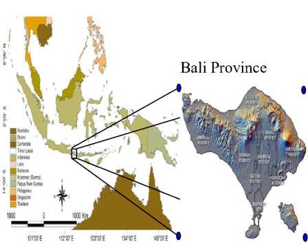
Figure 1. The Locations of the Research
each type of land use
|
Type of land use |
the runoff coefficient (Ci) |
|
Body of water |
0,8 (3) |
|
Building |
0,8 (3) |
|
0,06 | |
|
Forest |
(1) |
|
0,52 | |
|
Plantation |
(7) |
|
Mangrove |
0,3 (2) |
|
Sand |
0,1 (8) |
|
Beach sand |
0,1 (8) |
|
Settlement |
0,5 (6) |
|
Salinity |
0,8 (3) |
|
0,35 | |
|
Grasses |
(5) |
|
0,75 | |
|
Irrigated rice fields |
(3,4) |
|
0,52 | |
|
Rainfed lowland |
(4) |
|
0,35 | |
|
Bushes |
(2) |
|
Fishfond |
0,8 (3) |
|
Uncultivated Land |
0,2 (3) |
|
Moor / farm |
0,3 (5) |
Methodology
Calculation of Water Supply
The water supply calculation uses the runoff coefficient method, which is modified from the rational method. The calculation of equation of water supply of the runoff coefficient method is (Ministry of Environment, 2008):
SA = 10× C× R × A (1)
where SA is water supply (m3 / year), C is the weighted runoff coefficient, R is the average annual rainfall (mm / year), A is the size of area (hectare), and 10 is the conversion factor from mm/hectare to m3. Value of C is the average value of the coefficient of runoff in an area. In the year 2009, the value of the runoff coefficient was calculated by using the following equation (Ministry of Environment, 2009):
∑ (C1 × Ai) ∑ Ai
(2)
where Ci is the runoff coefficient of land use i (Table 1), while Ai is the area of land use i.
Table 1. The value of the runoff coefficient for
Sources: (1) Ward, A.D., S. T. Trimble (2004)
-
(2) Tunich-Nah Consultants & Engineering (2007)
-
(3) Jinno, et al. (2009)
-
(4) Yuge, et al. (2008)
-
(5) MoE (2008)
-
(6) Kadam, et al. (2009)
-
(7) The State of Queensland (2004)
In the year 2013, the value of the runoff coefficient was calculated by remote sensing approach. The calculation of the coefficient of runoff with remote sensing image analysis approach was effected by assuming the spectral values on the channels of remote sensing data which have a relationship with the imperviousness area (Schueler, 1994) as well as the condition and composition of vegetation density (Puigdefabregas 2005). In simple terms, the coefficient of runoff was related to the land cover types, through the capacity level of the types of land cover in infiltrating the surface water. In its approach to remote sensing, the area of imperviousness and the conditions and composition of vegetation density were obtained from the transformation of the Normalized Difference Vegetation Index (NDVI). NDVI (Tucker, 1979) is one of the very familiar indices used to map the distribution of vegetation rapidly,
and a variety of conditions on the surface of land. NDVI has a very strong relationship with the conditions and the density of vegetation (Carlson and Ripley, 1997; Purevdorj et al., 1998; Ishiyama et al., 2001; Glenn et al., 2008; As-syakur and Adnyana, 2009; Pettorelli et al., 2011). However, in addition to mapping the vegetated areas (quality and quantity), NDVI can also be used to map impervious areas. Matthias and Martin (2003) have always used NDVI to map impervious areas (imperviousness) in urban areas in Germany, whereas Wibowo and Yuniawati (2007) found a strong correlation between NDVI with imperviousness area percentage in the Citarum Hulu watershed. The transformation of the Landsat satellite imagery spectral values into NDVI uses the following equation (Tucker, 1979):
NDVI =
NIR - Red
NIR + Red
(2)
NIR is the channel near infrared wavelengths and Red is the red wavelength channel on the Landsat imagery. In this study, Landsat 8 was used in calculating the value of the runoff coefficient in the Bali Province.
The estimated runoff coefficient by the NDVI approach used three approaches: two approaches by equation and one approach by coefficients. The equation approaches, namely the equation of the NDVI value relationship with the percentage of imperviousness area and the equation of the NDVI value relationship with the percentage of vegetation density. In its analysis, if the value of NDVI <-0.0607, then it was transformed into a flow coefficient value based on the percentage of imperviousness area (Cip); if the NDVI values> 0.4202, then it was converted into flow coefficient value based on the vegetation density (Cvp); and if the NDVI values between -0.0607 to 0.4202, then the value of a given flow coefficient was at 0.4903. To find the value of the flow coefficient based on the percentage of imperviousness area, it was calculated by using equation (3), while to find the value of the flow coefficient based on the percentage of imperviousness area, it was calculated by using equation (4). The equations are as follows: (Wibowo and Hadi, 2008):
Cip = 0.05 + (0.91 * ((-63,61(NDVI)2 -
116,66(NDVI) + 46,977) /100))
(3)
Cvp = (- (127,19(NDVI) — 2,4779) / 100) + 1 (4)
In order to calculate the weighted average value of the runoff coefficient for each district, the raster data analysis results of remote sensing were truncated for each district by using the ArcView GIS software. Furthermore, the state of the average runoff coefficient per district was calculated by using the following equation:
CH
R = ^--j
JPijA
(5)
Where C is the average value of coefficient of runoff, CRij value is the value of the runoff coefficient on the pixelij (mm / year), and JPijA is the number of the pixelij in region A.
The average rainfall (R) was obtained from the analysis of the geographic information system (GIS) based on the annual rainfall data such as those used by Daryono (2002) in his research. The data were interpolated by using Kriging method of the Surfer 8.0 software. The interpolation was performed on the data of average annual rainfall in 58 rain posts in Bali Province; the data interval used was 10 to 22 years. In order to calculate the average rainfall per district, the raster data of interpolation were truncated for each district by using ArcView GIS software. After passing through the process of interpolation and truncation, the state of average annual rainfall per district was calculated by using the following equation:
CH
R = ^--i
JPijA
(6)
where R is the average rainfall (mm / year), the value of CHij is the rainfall on the pixelij (mm / year), and JPijA is the number of pixelij in region A.
Calculation of Water Demands
Calculation of the water demands in relation to the carrying capacity of water used the following equation (Ministry of Environment, 2008):
DA = N × KHL A (7)
where DA is the total water demand (m3 / year), N is the number of people (people), and KHLA is Falkenmark indicator which is the minimum water demands for decent living based on the estimated water demands of households, agriculture, industry and energy, as well as environmental demand (Falkenmark, 1989), in which the value assigned to Indonesia amounted to 1,600 m3 / capita / year (Ministry of Environment, 2008). The data of the population size per district of the Bali Province in 2008 and 2013 were obtained from the statistical books of ‘Bali Province in Figures’, year 2008 and 2013 (BPS, 2009, 2014).
Status Determination of Carrying Capacity of Water
The status of the carrying capacity of water is obtained from the comparison between the water supply (SA) and the water demand (DA) with the condition; SA > DA, the carrying capacity of water is declared to be a surplus, If SA < DA, the carrying capacity of water is declared to be a deficit (Prastowo et al., 2006).
Results and Discusion
Water Supply
The results of calculations showed that in 2009 and 2013 the supply of water for Bali Province amounted to 4.71 and 3.57 billion m3 / year. Specifically, in 2009, the supply of water for Tabanan was the largest, the supply of water in the year 2008 in the amount of 1.07 billion m3 / year, while the city of Denpasar was an area that had the lowest water supply, which amounted to 0.13 billion m3 / year. Whereas in 2013 the supply of water for Karangasem was the largest, amounting to 0.62 billion m3 / year, the city of Denpasar was an area that had the lowest water supply, which amounted to 0.10 billion m3 / year. The
level of water supply was influenced by three factors, namely rainfall, land cover type, and area. In 2009,Tabanan had a fairly high rainfall followed by a weighted runoff coefficient, the same condition also occurred in the year 2013 in Karangasem. In 2009 and 2013, the cities of Denpasar and Klungkung were among those with the lowest quantity of water supply. Denpasar City had the smallest level of water supply due to the small land area size as well as the high value of the weighted runoff coefficient. Klungkung had a low level of water supply due to the small amount of rainfall, especially in the subdistrict of Nusa Penida. The level of water supply for the Bali Province and districts in the Province of Bali can be seen in Table 2, while its distribution for Bali Province is presented in Figure 2.
Table 2. The size of area, the average rainfall, the average weighted runoff coefficient and the level of water supply in Bali in 2009 and 2013.
|
No |
District /City |
Size of Area (ha) |
Rainfall (mm/year) |
weighted runoff coefficient |
water supply (in billion of m3/year) | |||
|
2009 |
2013 |
2009 |
2013 |
2009 |
2013 | |||
|
District of Jembra |
84,1 80 |
1,726 |
1,869 |
0.34 |
0.22 |
0.49 |
0.34 | |
|
1 |
na Distri ct of Taba |
83,9 30 |
2,428 |
2,529 |
0.53 |
0.25 |
1.07 |
0.53 |
|
2 |
nan Distri ct of Badu |
42,0 09 |
2,033 |
2,035 |
0.48 |
0.35 |
0.41 |
0.30 |
|
3 |
ng Distri | |||||||
|
ct of Gian |
36,8 00 |
2,199 |
2,273 |
0.55 |
0.34 |
0.44 |
0.28 | |
|
4 |
yar Distri | |||||||
|
ct of |
31,5 00 | |||||||
|
Klun |
1,426 |
1,339 |
0.43 |
0.34 |
0.19 |
0.14 | ||
|
gkun | ||||||||
|
5 |
g Distri ct of Bang li |
52,0 81 |
2,219 |
2,171 |
0.44 |
0.35 |
0.51 |
0.40 |
|
6 |
1,989 |
2,158 |
0.42 |
0.34 |
0.70 |
0.62 | ||
|
Distri | ||||||||
|
ct of Kara |
83,9 54 | |||||||
|
ngase | ||||||||
|
7 |
m Distri ct of Bulel |
136, 588 |
1,727 |
1,750 |
0.36 |
0.23 |
0.85 |
0.55 |
|
8 |
eng | |||||||
|
City |
12,3 98 | |||||||
|
of Denp |
1,720 |
1,686 |
0.59 |
0.46 |
0.13 |
0.10 | ||
|
9 |
asar | |||||||
|
Provi | ||||||||
|
nce of |
563, 666 |
1,955 |
1,979 |
0.43 |
0.32 |
4.71 |
3.57 | |
|
10 |
Bali | |||||||
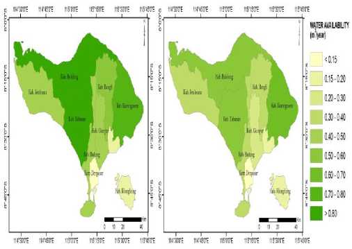
Figure 2. Distribution map of the amount of water supply per district in Bali for Year 2009 (left) and 2013 (right)
Water Demand
The total demand of water for the population of the Province of Bali in 2009 and 2013 reached 5.46 and 6.23 billion m3 / year. Water demand is increasing along with the increasing population number in the Province of Bali. In 2008, the highest level of water demand occurred in Buleleng which reached 1.04 billion m3 / year and Klungkung was the region with the lowest level of water consumption, which amounted to 0.28 billion m3 / year. The conditions in 2013 increased to 1.26 billion m3 / year in the City of Denpasar. In the meantime, Klungkung was the region with the lowest level of water consumption, which amounted to 0.27 billion m3 / year in the year of 2013. The high demand for water in the City of Denpasar was due to the large population. Based on the results of the 2010 census, the population of the City of Denpasar reached 788,589 inhabitants. The lowest water demand in Klungkung district was also due to its small population number. This suggests that the amount of water demand will increase along with the increasing number of population. The level of water demand for each district is presented in Table 3, and its distribution for the Province of Bali can be seen in Figure 3.
Table 3. The total population and the total water demand in Bali in 2009 and 2013
|
N o |
District/City |
Falkenmark Indicator |
Total of Populations (people) |
Water Demand (in billion of m3/year) | ||
|
2009 |
2013 |
2009 |
2013 | |||
|
Distric t of Jembr |
1.600 |
268, 269 |
0.43 |
0.42 | ||
|
1 |
ana District of |
1.600 |
416, 743 |
261,638 |
0.67 |
0.67 |
|
2 |
Tabanan |
420,913 | ||||
|
Distric t of Badun |
1.600 |
383, 880 |
0.61 |
0.87 | ||
|
3 |
g Distric t of Giany |
1.600 |
394, 755 |
543,332 |
0.63 |
0.75 |
|
4 |
ar Distric t of Klung |
1.600 |
176, 822 |
469,777 |
0.28 |
0.27 |
|
5 |
kung Distric t of |
1.600 |
213, 808 |
170,543 |
0.34 |
0.34 |
|
6 |
Bangli |
215,353 | ||||
|
Distric t of Karan |
1.600 |
430, 251 |
0.69 |
0.63 | ||
|
7 |
gasem Distric t of Bulele |
1.600 |
650, 237 |
396,487 |
1.04 |
1.00 |
|
8 |
ng City of Denpa |
1.600 |
475, 080 |
624,125 |
0.76 |
1.26 |
|
9 |
sar |
788,589 | ||||
|
Provin |
3,40 | |||||
|
ce of |
1.600 |
9,84 |
5.46 |
6.23 | ||
|
10 |
Bali |
5 |
3,890,757 | |||
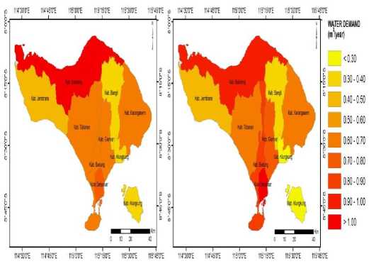
Figure 2. Distribution map of the amount of water demand per district in Bali for Year 2009 (left) and 2013 (right)
Status of Water Carrying Capacity
In general, the status of the water carrying capacity of Bali Province in 2009 was deficient with a status value below the carrying capacity of water or 0.86. Meanwhile, in 2013 the conditions also remained deficient, with the value of the carrying capacity declined to 0.57. The amount of water deficit in Bali in 2009 was 0.75 billion m3 / year, and increased to 2.65 billion m3 / year in 2013. The status of the water carrying capacity for each district in the Province of Bali in 2009 was quite evenly distributed between districts that experienced surplus status of water carrying capacity with those experiencing the deficit status of water carrying capacity. There were four districts which had the status of surplus water carrying capacity with values ranging from 1.59 to 1.02 or the amount of surplus water ranging from 0.40 to 0.01 billion m3 / year. On the other hand, there were five districts / cities that had a deficient carrying capacity of water ranging from 0.81 to 0.16 or the amount of water deficit ranging from 0.09 to 0.63 billion m3 / year. The district that had the highest surplus status of water carrying capacity was Tabanan and the city that experienced the highest deficit status of water carrying capacity was Denpasar.
Meanwhile in 2013, the status of the water carrying capacity for each district in the Province of Bali seemed to be uneven, with only one district that had a water surplus, namely the District of Bangli, whereas the remaining 8 districts / cities have experienced water deficit conditions. The District of Bangli has excess water of only 0.05 billion m3 / year, whereas the water deficit amounts of the eight districts / city range from 0.02 to 1.17 billion m3 / year. In detail, the value of the water carrying capacity and its status can be seen in Table 4 and Figure 4. The distribution of the value and the status of water carrying capacity of Bali Province is presented in Figure 5 and 6.
Under these conditions and in order to cope with the high rate of water deficit in the Province of Bali, it is necessary to reduce land conversion, especially the conversion of forests and agricultural areas into residential areas, because the impervious residential areas greatly affect the hydrological cycle in the
form of the infiltration process of rainwater into groundwater and the amount of surface runoff. This condition will affect the mainstay discharge which is part of the water supply. In addition, it is necessary for the restoration of forest areas as they serve orological functions, by controlling land use changes in forest areas, reforesting areas that have critical or very critical areas, as well as maintaining and overseeing the critical potential areas. Predicting the supply of water for the future also needs to be done, given the fluctuations in the water supply with a high enough variability of space and time.
Table 4. The value and the status of water carrying capacity of Bali Province
|
N u m. |
District/City |
Value of the carrying capacity of water |
Status of the carrying capacity of water | ||
|
2009 |
2013 |
2009 |
2013 | ||
|
1 |
District of Jembrana |
1.15 |
0.82 |
Surplus |
Deficit |
|
2 |
District of Tabanan |
1.59 |
0.79 |
Surplus |
Deficit |
|
3 |
District of Badung |
0.67 |
0.35 |
Deficit |
Deficit |
|
4 |
District of Gianyar |
0.70 |
0.37 |
Deficit |
Deficit |
|
5 |
District of Klungkung |
0.68 |
0.53 |
Deficit |
Deficit |
|
6 |
District of Bangli |
1.48 |
1.16 |
Surplus |
Surplus |
|
7 |
District of Karangasem |
1.02 |
0.98 |
Surplus |
Deficit |
|
8 |
District of Buleleng |
0.81 |
0.55 |
Deficit |
Deficit |
|
9 |
City of Denpasar |
0.16 |
0.08 |
Deficit |
Deficit |
|
10 |
Province of Bali |
0.86 |
0.57 |
Deficit |
Deficit |
■ 2009 ■ 2013
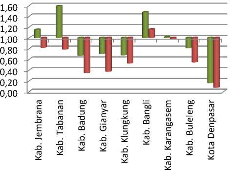
Figure 4. The graph of values, and the status of the water carrying capacity of Bali Province.
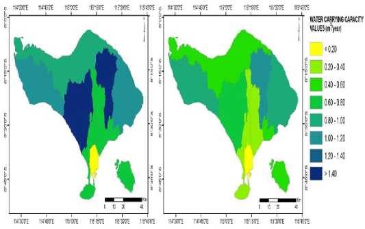
Figure 5. Distribution map of carrying capacity of water per district in Bali
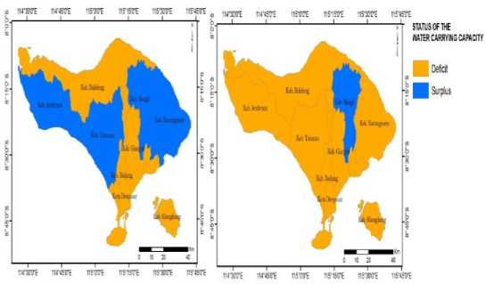
Figure 6. Distribution map of the status of water carrying capacity of Bali Province in 2009 (left) and 2013 (right)
Conclusion and Recommendation
The calculation shows that the total water supply of the island of Bali in 2009 amounted to 4.71 billion m3 / year and decreased to 3.57 billion m3 / year in 2013. During that period, the total water demand increased, in which in 2009 it was at 5.46 billion m3 / year, and in 2013 amounted to 6.23 billion m3 / year. Thus, the island of Bali in 2009 and in 2013 experienced a water deficit. The condition of the island of Bali in 2009 showed that of the 9 districts / cities, five of them experienced water shortages with the amount of water deficit ranging from 0.09 to 0.63 billion m3 / year. Whereas in 2013, it amounted to 8 districts / cities that experienced a water deficit which ranged from 0.02 to 1.17 billion m3 / year. Therefore, Bali should take serious
steps to save water resources, not only to save tourism development which is a mainstay of the island of Bali, but also the sustainability of the Balinese people’s lives.
References
Aldrian, E. and Dwi Susanto, R. (2003) ‘Identification of three dominant rainfall regions within Indonesia and their relationship to sea surface temperature’, International Journal of Climatology. Wiley Online Library, 23(12), pp. 1435–1452.
As-syakur, A. R. (2010) ‘Pola spasial pengaruh kejadian La Nina terhadap curah hujan di Indonesia tahun 1998/1999; observasi menggunakan data TRMM Multisatellite
Precipitation Analysis (TMPA) 3B43’, Dalam prosiding Pertemuan Ilmiah Tahunan (PIT) XVII dan Kongres Masyarakat Penginderaan Jauh Indonesia (MAPIN) V. Institut Pertanian Bogor, 9, pp. 230–234.
As-syakur, A. R. et al. (2013) ‘Indonesian rainfall variability observation using TRMM multi-satellite data’,
International journal of remote sensing. Taylor & Francis, 34(21), pp. 7723–7738.
As-syakur, A. R. and Adnyana, I. W. S. (2009) ‘Analisis indeks vegetasi
menggunakan citra ALOS/AVNIR-2 dan sistem informasi geografi (SIG) untuk evaluasi tata ruang kota Denpasar’, Bumi Lestari, 9(1), pp. 1– 11.
As-syakur, A. R. and Prasetia, R. (2010) ‘Pola spasial anomali curah hujan selama Maret sampai Juni 2010 Di Indonesia; Komparasi data TRMM Multisatellite Precipitation Analysis (TMPA) 3B43 dengan stasiun pengamat hujan’, Prosiding Penelitian Masalah Lingkungan di Indonesia 2010; Buku, 2, p. 29.
BPS (2009) Provinsi Bali dalam Angka 2008. Denpasar: Badan Pusat Statistik
Provinsi Bali.
BPS (2014) Provinsi Bali dalam Angka 2013. Denpasar: Badan Pusat Statistik
Provinsi Bali.
Carlson, T. N. and Ripley, D. A. (1997) ‘On the relation between NDVI, fractional vegetation cover, and leaf area index’, Remote sensing of Environment.
Elsevier, 62(3), pp. 241–252.
Daryono (2002) Identifikasi Unsur Iklim, Sifat Hujan, Evaluasi Zone Iklim Oldeman dan Schmidt-Fergiuson Daerah Bali Berdasarkan Pemutakhiran Data.
Universitas Udayana.
Daryono (2004) ‘Iklim Bali Ditinjau dari Peta Isohyets Normal Curah Hujan’, Jurnal Meteorologi dan Geofisika, 9, pp. 14– 19.
Falkenmark, M. (1989) ‘The massive water scarcity now threatening Africa: why isn’t it being addressed?’, Ambio. JSTOR, pp. 112–118.
Glenn, E. P. et al. (2008) ‘Relationship between remotely-sensed vegetation indices, canopy attributes and plant physiological processes: what
vegetation indices can and cannot tell us about the landscape’, Sensors. Molecular Diversity Preservation International, 8(4), pp. 2136–2160.
Ishiyama, T. et al. (2001) ‘Relationship among vegetation variables and vegetation features of arid lands derived from satellite data’, Advances in Space Research. Elsevier, 28(1), pp. 183– 188.
Jin, Z. (2006) ‘A Discussion about the Problems on Water Resources Carrying Capacity Research’, in
roceeding of GMSARN International Conference on Sustainable
Development: Issues and Prospects for GMS, pp. 1–5.
Matthias, B. and Martin, H. (2003) ‘Mapping imperviousness using NDVI and linear spectral unmixing of ASTER data in the Cologne-Bonn region (Germany)’, in Proc. SPIE, pp. 274–284.
Pettorelli, N. et al. (2011) ‘The Normalized Difference Vegetation Index (NDVI): unforeseen successes in animal ecology’, Climate Research. JSTOR, 46(1), pp. 15–27.
Prastowo, H. et al. (2006) Kajian Daya Dukung Lingkungan DAS Siak Sebagai Salah Satu Acuan Percontohan Dalam Penyusunan
Pedoman Perhitungan Daya Dukung Lingkungan. Jakarta: Kementrian
Negara Lingkungan Hidup Republik Indonesia.
Purevdorj, T. S. et al. (1998) ‘Relationships between percent vegetation cover and vegetation indices’, International journal of remote sensing. Taylor & Francis, 19(18), pp. 3519–3535.
Schueler, T. R. (1994) ‘The importance of imperviousness’, Watershed
protection techniques, 1(3), pp. 100– 111.
Silvers, J. R. (2007) ‘Analysis of the international EMBOK model as a classification system’, in Las Vegas International Hospitality and
Convention Summit. Las Vegas: University of Nevada.
Suyono, T. et al. (2006) ‘Kajian Daya Dukung Daerah Aliran Sungai Babon-Jawa Tengah (sebagai salah satu acuan percontohan dalam menyusun pedoman perhitungan Daya Dukung Lingkungan)’. Jakarta: Kementrian Negara Lingkungan Hidup Republik Indonesia.
Tucker, C. J. (1979) ‘Red and photographic infrared linear combinations for monitoring vegetation’, Remote sensing of Environment. Elsevier, 8(2), pp. 127–150.
Wibowo, H. and Hadi, M. P. (2008) ‘Transformasi NDVI untuk estimasi nilai koefisien aliran:: Kasus aplikasi Citra Landsat ETM+ di DAS Citarum Hulu’. Universitas Gadjah Mada.
Wibowo, L. A. and Yuniawati, Y. (2007) ‘The Influence of Tourist Product Attribute and Trust to Tourist Satisfaction and Loyalty A Study of Mini Vacation in Bandung’, Ringkasan Hasil Penelitian Dosen.
http://ojs.unud.ac.id/index.php/eot
42
e-ISSN: 2407-392X. p-ISSN: 2541-0857
Discussion and feedback