IDENTIFICATION OF SHORELINE CHANGES USING SENTINEL 2 IMAGERY DATA IN CANGGU COASTAL AREA
on
Identification of Shoreline Changes Using Sentinel 2 Imagery Data In Canggu Coastal Area
[Sagung Putri dkk.]
IDENTIFICATION OF SHORELINE CHANGES USING SENTINEL 2 IMAGERY DATA IN CANGGU COASTAL AREA
Sagung Putri Chandra Astiti1*), Takahiro Osawa2,3), I Wayan Nuarsa4) 1)Master Degree Program of Environmental Science Udayana University 2)Center for Remote Sensing and Ocean Sciences (CReSOS) Udayana University 3)Center for Research and Application of Satellite Remote Sensing (YUCARS) Yamaguchi University 4) Doctoral Program of Environmental Science Udayana University
*Email: sagungchandra17@gmail.com
ABSTRACT
Coastal areas in the Canggu and Seminyak areas located in Badung Regency, Bali Province are very attractive tourism. The development of tourism has an impact on coastal conditions. The coastal conditions analyzed are changes in coastline that occurred during 2015-2019 using remote sensing. The satellite image data used in the analysis is Sentinel 2A image data that can be accessed for free with a spatial resolution of 10 meters. Image data processing is divided into three stages, namely preprocessing, processing, and post processing using Sentinel Application Platform (SNAP) software. The preprocessing stage includes the resampling, masking, and subset areas. The processing stage includes digitizing the coastal area, digitizing accuracy analysis using the Support Vector Machine (SVM) method, and the post processing stage including correction of shoreline changes. Bands in image data used for detection of coastal areas are band 8 (NIR), 8A (narrow NIR), 11 (SWIR), and 12 (SWIR). Based on the results of the analysis of shoreline changes carried out during 2015-2019, it was found that the average shoreline changes were 1.42 m / year with erosion conditions in which the dominant wind direction originated from the southwest towards the northeast coast of the sea of Bali. The results of digitizing the coastal area using the Fine Gaussian SVM method with the greatest accuracy value is 87.8%.
Keywords: Shoreline Change, Remote Sensing, Sentinel 2A, SVM, Wind Direction
Natural phenomena such as wind, waves, tides, sediment flows and transportation that occur continuously in coastal areas will cause a dynamic of coastal areas in the form of shoreline changes. Shoreline changes occur because the coastal area experiences pressure and causes various problems in the coastal environment. Erosion and accretion that occur in coastal areas is one sign of changes in coastline. According to Triatmodjo (1999), sediment transport that occurs in coastal areas causes changes in coastline. Sediment transport carries material from various sources such as the sea and rivers caused by currents so that erosion and accretion occur. In addition
to natural phenomena, shoreline changes can occur due to anthropogenic activities caused by humans. According to Shuhendry (2004) in Halim et al (2016), activities that can affect the occurrence of shoreline changes are land conversion and conversion of coastal protection lands to support tourism activities that are not in accordance with the applicable rules so that the balance of sediment transport can be disrupted, currents and waves triggered by sand mining.
The beach in the Canggu Region, North Kuta Subdistrict, Badung Regency has the potential to be used for the development of tourism areas because of the characteristics of the beach which has large waves so that it is used for surfing activities, especially foreign tourists. Beaches in Canggu include Berawa Beach, Nelayan
Beach, Canggu Beach, Batu Bolong Beach, Batu Mejan Beach, Pererenan Beach and Seseh Beach. In addition to tourism activities, the coastal area is also used for religious ritual activities by the surrounding community. Beaches in the Canggu area have coral clusters in certain positions and have black beach sand due to the influence of sediment carried from rivers in coastal areas to be discharged into the sea. Beach buildings are already in several positions but some are damaged due to large waves. The beach building was used to protect the temple in the coastal area of Canggu for religious rituals.
There are several natural vegetative to protect coastal areas, but the vegetative amount is still very lacking so that the coastal safeguards in this area need to be optimized. The implementation of coastal protection buildings to withstand large waves is not yet found on the beach in the Canggu area. Beach abrasion in the Canggu area can be seen with beach shifts that are starting to approach tourism supporting buildings such as restaurants and bars.Based on the Report on Coastline Change Analysis of the Balai Wilayah Sungai Bali - Penida (BWS Bali-Penida), the results of erosion rates in 1999-2009 were 1.75 m/year and in 2009-2015 were 1.96 m/year in Canggu Area, North Kuta District, Badung Regency. In the report, it was stated that Badung Regency was the fourth priority area for handling erosion among regencies or cities located on the island of Bali.
Seeing this problem, the authors want to know the changes in the coastline that occurred in 2015 - 2019 through Sentinel 2 Imagery Data. The use of satellite imagery in shoreline change research is needed because in satellite image data there is an image recording date that provides information about tidal time events in the study year to be analyzed. Sentinel 2 satellite image data is used because the data can be accessed for free and has a spatial resolution of 10 x 10 meters that is better than Landsat TM satellite imagery. According to Illahude (2009), ocean waves and currents included in oceanographic parameters are generated by surface wind so that the rate of erosion and increase that occurs is influenced by these parameters. Based on the statement, the author wanted to analyze the relationship between wind direction and the rate of change in coastline that occurred at the study site.
The research locations are in the coastal areas of Canggu and Seminyak located in Badung Regency, Bali Province to conduct coastline change research using Sentinel 2A satellite image data from 2015 to 2019 by recording the best quality image data per year. For wind direction analysis, the data used is Sentinel 1A satellite image data GRDH Level which is analyzed per month during the study year.
Table 1. Research Data Sources
|
No Data |
Source |
|
1 Sentinel 2A recording on December 23th, 2015 2 Sentinel 2A recording on October 25th, 2016 3 Sentinel 2A recording on July 2nd, 2017 4 Sentinel 2A recording on April 18th, 2018 5 Sentinel 2A recording on February 2nd, 2019 6 Sentinel 1A 2015-2019 |
https://scihub.copernicus.euhttps://scihub.copernicus.eu https://scihub.copernicus.euhttps://scihub.copernicus.eu https://scihub.copernicus.euhttps://asf.alaska.edu |
|
No |
Data |
Source |
|
7 |
Digital Elevation Mode (DEM) Data | |
|
8 |
Tidal Data |
Tides Application |
|
9 |
Wind Speed Data | |
|
10 |
Survey the Research Area |
Field Observation |
Preprocessing image data is a preanalysis of satellite image data that aims to improve the quality of satellite image data, eliminate noise in image data, improve image, transform images and determine the part of the image to be used. The preprocessing stage in satellite image data includes resampling data images, geometric correction, atmospheric correction, masking and subset image data.
The process of processing pixels in a digital image to obtain information contained in an image is the definition of image processing. Image processing is grouped into two types, namely processing information contained in the image and improving the image in accordance with the requirements. In this study, included in the stages of image processing are unsupervised classification, pixel classification learner and shoreline change model.
Pixel classification using MATLAB is one of the classification models using machine learner, where the classification uses bands in satellite imagery used for sand classification. The bands used in the classification of sand in Sentinel 2A are
band 8 (NIR), band 8A (Narrow NIR), band 11 (SWIR) and band 12 (SWIR). After that, MATLAB software will study the pixel values and classify them based on the range of values for the type of black sand and white sand.
A stage that aims to increase the accuracy of processing results from satellite image data is called the post processing stage. Post processing stages included in this study are tidal correction stages to get a more accurate shoreline change. The aim of tidal correction in the analysis of shoreline changes is to correct changes in the gravitational field values on the earth's surface due to the attraction of the earth by the moon and the sun. Therefore, tidal correction is very dependent on the position of the moon and sun on the earth. The data needed in tidal correction include HWL data at the study site, HWL data at Benoa station and slope data at the study site. After tidal correction is carried out, the next step is to make a transect to determine the shoreline changes at each transect point. In this study, 100 transects were analyzed for shoreline changes.
-
3. RESULT AND DISCUSSION
3.1 Preprocessing Result
-
(a) (b)
-
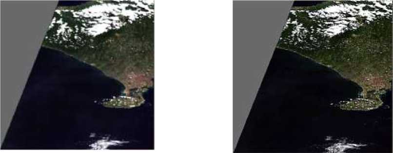
Figure 1.
Sentinel 2A Imagery Satellite After Being Implemented by Resampling Respectively: a) Before Resampling and b) After Resampling Process
Resampling is a process that changes the value of the original raster pixel (domain) to a result raster pixel value (codomain). In this study using the nearest neighbor method that makes every band that responding experienced a change in pixel size where Sentinel 2A images had three
different resolutions in each band and then made one resolution which was the highest resolution with a value of 10 m. The pixel size is in the image resolution of 20m and 60m which was originally large after it was done the resampling process will result in smaller pixel sizes.

(a) (b)
-
Figure 2.
Sentinel 2A Imagery Satellite After Being Implemented by Masking
Respectively: a) Before Masking and b) After Masking Process
The process for determining the spatial boundary between clouds and not clouds is the process of cloud masking. The method used to separate clouds is to determine the threshold value in the blue
band (BOA reflectance) Sentinel-2A image. Thresholding is the simplest method of image segmentation. The result of the process is a binary image, where the cloud will be 0 and not the cloud will be worth 1.
(a)
(b)
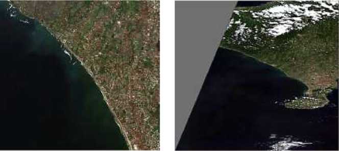
Figure 3.
Sentinel 2A Imagery Satellite After Being Implemented by Subset Respectively: a) Before Subset and b) After Subset Process
Subset is one step to reduce the time in the process of image data by focusing image data in the field of research used so that it will facilitate analysis activities. In the subset menu, there are settings for selecting
the coordinates of Area Of Interest (AOI) as needed by entering values in each scene. The scene used are scene start x (8944), scene start y (5526), scene end x (9986), and scene end y (6287).

-
(a) (b)
-
Figure 4.
Sentinel 2A Imagery Satellite After Being Implemented by Unsupervised Classification
Respectively: a) Before Classification and b) After Unsupervised Classification
In this study, image data are grouped into two classes, namely black sand class and white sand class. The selection of the class is based on the condition of the sand found in the research area where this research is located, the starting point of the location is Mengening Beach, which is the border area between Badung Regency and
Tabanan Ragency and the location endpoint is in the Seminyak area. Mengening Beach and the Canggu area beach have the characteristics of black sand while the beaches of the Seminyak area have the characteristics of white sand.
After the digital number value is studied by MATLAB software, then the
program will predict the value of the digital number produced as a class of white sand or black sand. The results of these predictions are obtained by entering the programming language yfit= C.predictFcn(T).
After the classification results are obtained, the next step is to get a scatter plot and confusion matrix diagram from MATLAB software. The type of SVM method used is Fine Gaussian SVM because the accuracy of the results of the data obtained is very high at 87.8%. The results of the scatter plot and confusion matrix diagram are shown in Figure 5 and Figure 6.

Figure 5.
Scatter Plot Result
Scatter plots function to see the accuracy of relationships between variables that are needed and help to determine the type of equation that will be used to determine the relationship. In Figure 5, the relationship between band 8 and band 8A was analyzed so that the scatter plot was
obtained. The blue color shows scatter plots of black sand and orange colors showing scatter plots of white sand. The values that are classified as the type of sand that is less precise will be symbolized by the cross shape and the actual classification color.
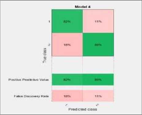
Figure 6.
Confusion Matrix Result
The Confusion Matrix in MATLAB serves to provide information from the processing of training data obtained, to provide an assessment of the results of machine learning classification based on objects that are accurately and inappropriately classified and there is actual information and predictive information on the classification system. Based on the results of the Confusion Matrix in MATLAB, it was found that the pixel value of digitizing black sand that was correctly classified as 82 % and 18 % of the pixel value was classified incorrectly. Whereas for pixel values from digitizing white sand which are classified correctly, 89 % and 11 % of pixel values are classified incorrectly

Figure 7.
Shoreline Change Graph Result
After the accuracy of the data value of the digital number was tested using MATLAB, the next step is to enter the digital number value into Excel format to get a graph of the shoreline change in the study area. Based on Figure 7 above, the results of the shoreline changes for 20152019 are distinguished based on the color of the lines representing each year.
The red color shows the coastline based on the recording of satellite image data on 31 December 2015, yellow indicates the coastline based on the recording of satellite image data on 25 October 2016, green indicates the coastline based on recording satellite image data on 02 July 2017, the blue color shows the coastline based on the recording of satellite image data on April 18, 2018 and the orange color shows the coastline based on the recording of satellite image data on 02 February 2019. The selection of image recording data for each year is based on the smallest cloud cover conditions in the study location analyzed.
After the graph of the coastline change is obtained, the next step is to analyze the slope of the land in the area that has been digitized. The analysis includes geoprocessing processes, spatial analysis processes and converting the results of spatial analysis in the form of excel. Spatial analysis has a very important role because spatial analysis methods can combine raster data with vector data and spatial analysis provides tools to create surface areas and analyze characteristics such as slope. The function of slope in spatial analysis is to determine the rate of change of each image cell analyzed and produce a slope grid that can be either a percentage unit or a degree unit. The example of slope results using the spatial analysis method are shown in Figure 8.
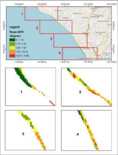
Figure 8.
Slope Result
The step that aims to improve the accuracy of the processing results from satellite image data is called the post processing stage. The post-processing stage included in this study is the tidal correction stage to get a more accurate change in coastline. Examples of shoreline correction calculations and shoreline change charts that include tidal correction calculations will be shown in Figure 9.
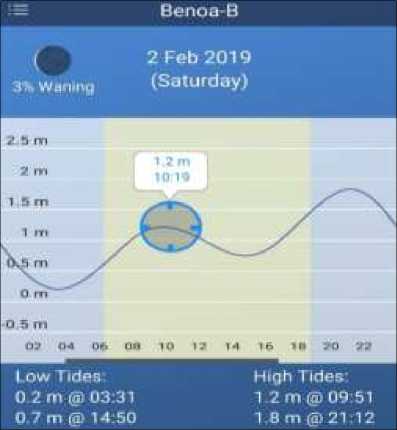
Figure 9.
Tides Data
Data needed to calculate tide correction are high water lever data at the study site, high water level data at the closest station to the study site, and tidal height data at the time of image recording. The closest station to the study site is Benoa Station and the image recording time on February 2nd, 2019 is 10: 19 A.M. The data is obtained through the Tides application and then the data is analyzed to perform calculations by entering the following formula.
Y = (Tk - (½ x Tx) x Tan 0) (1)
Based on the data obtained, the following information is obtained.
High water level at the study site (Tk) = 1.8m
High water level at Benoa Station (Tb) = 1.8m
Tidal Altitude at image recording time = 1.2m
The slope value is adjusted to the transect analyzed.
Then it is obtained,
Y = (1.8 — (l8 x 1'2)x Tan (3-24)) = 1.372 m ’
Based on the average yield of each transect of coastline changes during 20152016 there was erosion of 4.39 m while for the average yield of each transect of coastline changes during 2016-2017 erosion was 3.16 m, the average yield of each line transect the coast changes during 2017-2018 accretion occurred at 1.71 m and the the average yield of each line transect the coast changes during 2018-2019 accretion occurred at 0.16 m . The average yield of each transect during 2015-2019, the results showed that erosion was 1.42 m/year at the study site. This result does not deviate too much from reports of changes in shoreline carried out by Balai Wilayah Sungai (BWS) before the study year, during 2009-2015 erosion was 1.96 m/year.
Wind is a major factor in the movement of currents and waves, thus providing a large distribution of shoreline changes that occur in the study area. Winds that blow both from the sea to land and vice versa occur due to differences in temperature and humidity. Waves generated due to the movement of winds that pass through the sea surface have different strengths depending on the speed. Wind can
also cause currents along the coast if the direction follows the direction of the wind that blows around the beach. The wind that blows throughout the year and has a different direction twice a year is called the Monsoon wind. The characteristic of the Monsoon season is the difference between the wet season and the dry season, where the wet season occurs in the December, January and February (DJF) periods, while the dry season occurs in the June, July and August periods (JJA).
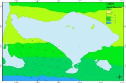
Figure 10.
Wind Direction in the Rainy Season in the Bali Sea Region
During the rainy season which lasts during December, January and February during 2015, the speed and direction of the wind produced varies. In January, the wind direction came from the southwest to the northeast with wind speeds ranging from 5 – 5.9 m/s while in February, the wind direction came from the south to the northeast with wind speeds ranging from 2.1 – 2.9 m/s and in December, the wind direction comes from west to southeast with wind speeds ranging from 2 – 2.9 m/s. The results of the analysis in 2016 also showed varied results. In January, the wind direction comes from the west to the southeast with an average wind speed of 1.1 – 2.1 m/s, whereas in February, the wind direction comes from the southwest to the northeast with an average wind speed of 3.3 – 4.2 m/s and in December, the wind direction is from
west to east with an average wind speed of 1.2 – 2.1 m/s.
For the results of analysis during 2017-2018, the rainy season shows almost the same results for wind direction. In 2017 in January, the wind direction comes from west to east with wind speeds ranging from 3.1 to 4 m/s while in February, the wind direction comes from southwest to northeast with wind speeds starting at 7.1 – 8 m/s and in December, the wind direction from west to east with wind speeds ranges between 3.1 – 4 m/s. In 2018, the wind direction came from west to east in January with wind speeds ranging from 1.1 – 2 m/s, while in February, the wind direction came from west to east with wind speeds ranging from 4.1 – 5 m/s and in December, the wind direction comes from the southwest to the northeast with wind speeds ranging from 3.1 – 4 m/s

Figure 11.
Wind Direction in the Wet Season in the Bali Sea Region
In the dry season that occurs in June, July and August, the wind direction generated is relatively constant for the year of analysis during 2015-2018. For 2015 in June and July, the wind direction comes from west to east with wind speeds ranging from5 – 5.9 m/s in June and 6 – 6.9 m/s in July. In August, the wind direction came from northwest to southeast with wind speeds ranging from 6 – 6.9 m/s. In 2016, wind direction in June, July and August came from west to east with wind speeds ranging from 3.3 – 4.2 m/s in June, 2.2 – 3.2 m/s in July and 5.4 – 6.3 m/s in August.
In 2017 in June and July, the wind direction comes from the southwest to the northeast with wind speeds ranging from 6.1 – 7 m/s in June and 3.1 – 4 m/s in July whereas in August, the wind direction came from west to east with wind speeds ranging from 6.1 – 7 m/s. In 2018, the wind direction came from west to east with wind
speeds ranging from 4.1 – 5 m/s in June while for July and August, the wind direction came from southwest to northeast with wind speeds ranging from 6.1 – 7 m/s in July and 4.1 – 5 m/s in August.
Estimation of wave height at the study site is obtained based on the length of the fetch in the study area with the wind speed at sea obtained at the study site. To get the effective length of the fetch, the steps that need to be done are to make the angle increase ranging from 60 to 420 degrees. The addition of angles in the form of lines be displayed in Figure 12 and the results of the calculation of the effective fetch length will be displayed on Table 2. The results of the calculation of the wind stress factor will be shown in Table 3.
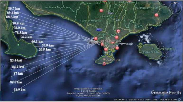
Figure 12.
Effective Fetch Length
|
Table 2. Effective Fetch Calculations | |||
|
Angle (α) |
Cos α |
Distance (Xi) Km |
Xi.cos α |
|
42 |
0.74 |
89.7 |
66.66 |
|
36 |
0.81 |
89.3 |
72.25 |
|
30 |
0.87 |
88.3 |
76.47 |
|
24 |
0.91 |
80.9 |
73.91 |
|
18 |
0.95 |
78.9 |
75.04 |
|
12 |
0.98 |
78.5 |
76.78 |
|
6 |
0.99 |
76.2 |
75.78 |
|
0 |
1.00 |
66.1 |
66.10 |
|
6 |
0.99 |
57.9 |
57.58 |
|
12 |
0.98 |
56.9 |
55.66 |
|
18 |
0.95 |
83.4 |
79.32 |
|
24 |
0.91 |
84.9 |
77.56 |
|
30 |
0.87 |
87 |
75.34 |
|
36 |
0.81 |
89.8 |
72.65 |
|
42 |
0.74 |
92.9 |
69.04 |
|
Total |
13.51 |
1070.14 | |
|
Feff |
79.21 | ||
Table 3. Wind Stress Factor Calculation
|
Month |
Wind Stress Factor (Ua) |
Feff (Km) |
Wave Height (m) |
Period (s) |
|
Jan-15 |
7.26 |
79.21 |
1.03 |
5.2 |
|
Feb-15 |
2.57 |
79.21 |
- |
- |
|
Mar-15 |
5.08 |
79.21 |
0.72 |
4.7 |
|
Apr-15 |
5.29 |
79.21 |
0.76 |
4.8 |
|
May-15 |
1.77 |
79.21 |
- |
- |
|
Jun-15 |
6.82 |
79.21 |
0.98 |
5.1 |
|
Month |
Wind Stress Factor (Ua) |
Feff (Km) |
Wave Height (m) |
Period (s) |
|
Jul-15 |
8.91 |
79.21 |
1.25 |
5.5 |
|
Aug-15 |
9.59 |
79.21 |
1.38 |
5.7 |
|
Sep-15 |
7.79 |
79.21 |
1.12 |
5.3 |
|
Oct-15 |
6.01 |
79.21 |
0.88 |
4.8 |
|
Nov-15 |
4.66 |
79.21 |
0.72 |
4.7 |
|
Dec-15 |
3.88 |
79.21 |
- |
- |
|
Jan-16 |
2.11 |
79.21 |
- |
- |
|
Feb-16 |
7.49 |
79.21 |
1.06 |
5.3 |
|
Mar-16 |
5.13 |
79.21 |
0.74 |
4.7 |
|
Apr-16 |
5.25 |
79.21 |
0.76 |
4.7 |
|
May-16 |
5.19 |
79.21 |
0.74 |
4.7 |
|
Jun-16 |
4.79 |
79.21 |
0.72 |
4.7 |
|
Jul-16 |
5.74 |
79.21 |
0.82 |
4.8 |
|
Aug-16 |
9.79 |
79.21 |
1.42 |
5.7 |
|
Sep-16 |
7.25 |
79.21 |
1.03 |
5.2 |
|
Oct-16 |
1.39 |
79.21 |
- |
- |
|
Nov-16 |
4.76 |
79.21 |
0.72 |
4.7 |
|
Dec-16 |
1.89 |
79.21 |
- |
- |
|
Jan-17 |
4.18 |
79.21 |
- |
- |
|
Feb-17 |
8.08 |
79.21 |
1.18 |
5.4 |
|
Mar-17 |
2.48 |
79.21 |
- |
- |
|
Apr-17 |
3.40 |
79.21 |
- |
- |
|
May-17 |
4.18 |
79.21 |
- |
- |
|
Jun-17 |
8.66 |
79.21 |
1.25 |
5.5 |
|
Jul-17 |
4.20 |
79.21 |
- |
- |
|
Aug-17 |
7.21 |
79.21 |
1.03 |
5.2 |
|
Sep-17 |
5.97 |
79.21 |
0.88 |
4.8 |
|
Oct-17 |
7.26 |
79.21 |
1.04 |
5.2 |
|
Nov-17 |
3.49 |
79.21 |
- |
- |
|
Dec-17 |
5.14 |
79.21 |
0.73 |
4.7 |
|
Jan-18 |
1.74 |
79.21 |
- |
- |
|
Feb-18 |
7.94 |
79.21 |
1.14 |
5.3 |
|
Mar-18 |
1.47 |
79.21 |
- |
- |
|
Apr-18 |
1.52 |
79.21 |
- |
- |
|
May-18 |
7.07 |
79.21 |
1 |
5.2 |
|
Jun-18 |
4.54 |
79.21 |
0.72 |
4.7 |
|
Jul-18 |
9.01 |
79.21 |
1.26 |
5.6 |
|
Aug-18 |
8.06 |
79.21 |
1.16 |
5.3 |
|
Sep-18 |
5.97 |
79.21 |
0.88 |
4.8 |
|
Oct-18 |
3.91 |
79.21 |
- |
- |
|
Nov-18 |
3.44 |
79.21 |
- |
- |
|
Dec-18 |
4.95 |
79.21 |
0.72 |
4.7 |
|
Jan-19 |
2.52 |
79.21 |
- |
- |
|
Feb-19 |
4.83 |
79.21 |
0.72 |
4.7 |
-
1. The results of the analysis for shoreline changes in the study area showed that erosion was 1.42 m/year using Sentinel 2A image data in this study are during 2015-2019. Based on the results of the wind direction analysis carried out during the study year, namely 2015-2019, wind direction results indicate that the wind direction that evokes ocean waves in the Bali sea area generally originates from the southwest to the northeast with varying wind speeds. The results showed that the wind speed in the dry season that occurs in June, July and August is greater than the wind speed in the rainy season which occurs in December, January and February. Based on the results of the wind direction analysis carried out during the study year, namely 2015-2019, wind direction results indicate that the wind direction that evokes ocean waves in the Bali sea area generally originates from the southwest to the northeast with varying wind speeds. The results showed that the wind speed in the dry season that occurs in June, July and August is greater than the wind speed in the rainy season which occurs in December, January and February.
-
2. The movement of the wind direction can affect the direction of erosion and the movement of sediments and to achieve a shoreline balance, generally at some point there be erosion and another point accretion. Based on the results of the analysis found that the average wave height affects the shape of the resulting coastline changes. The average wave height of December 2015 has 0.34 m, October 2016 has 0.75 m, July 2017 has 1.14 m, April 2018 has
0.41 m and February 2019 has 0.42 m. There was found that the erosion conditions occurred in 2015 - 2016 and in 2016 - 2017, while the
accretion conditions occurred in 2017 - 2018. The coastline
conditions in 2018-2019 were stable.
-
1. To perfect this research, it is necessary to analyze changes in coastline for a long period of time, for example for a range of 10 years. The research carried out in this report was only carried out during 2015-2019 because the author used Sentinel 2A satellite image data which began operations in 2015. The use of Sentinel 2A satellite image data was used because the image has a resolution of 10 meters with data that can be accessed for free. The detection of wind direction that generates waves is only analyzed based on wind direction obtained from recording Synthetic Aperture Radar (SAR) image data, which is during the 2015-2019 recording year. To find out more detailed wave directions, it can be done by doing wave modeling by collecting the required data.
-
2. The detection of wind direction that generates waves is only analyzed based on wind direction obtained from recording Synthetic Aperture Radar (SAR) image data, which is during the 2015-2019. To find out more detailed wave directions, it can be done by doing wave modeling by collecting the required data. The coastline changes produced in the analysis obtained are only reviewed based on the average wave height produced. To get the results of a more optimal influence analysis, it must be reviewed based on land influences such as the effect of river discharge generated in each season
so that the sea influence and land influence have a balance for shoreline changes that occur in the study area. Weaknesses in this study are also found in recording satellite image data obtained per year, where recording satellite imagery does not
REFERENCES
Aryastana,P.,Ardantha,
I.M.,Agustini,N.K.A. 2017.Analisis
Perubahan Garis Pantai dan Laju Erosi di Kota Denpasar dan Kabupaten Badung Dengan Citra Satelit SPOT. Bali, Indonesia : Universitas
Warmadewa. . Jurnal Fondasi, 6(2)
:100 – 111.
Darwin, Pinem, M., Simanjuntak, M.A. 2017. Analisis Perubahan Garis Pantai Menggunakan Citra Penginderaan Jauh (Studi Kasus di Kecamatan Talawi Kabupaten Batubara). Medan, Indonesia : Universitas Negeri Medan. Jurnal Geografi, p. 21-31
Fletcher, K. 2012. Sentinel-2 ESA’s Optical High-Resolution Mission for GMES Operational Services. Netherlands : ESA Communications.
Halim, Halili, Afu, LOA. 2016. Studi Perubahan Garis Pantai Dengan Pendekatan Penginderaan Jauh di Wilayah Pesisir Kecamatan Soropia. Palu, Indonesia : Universitas Halu Oleo. Sapa Laut, 1(1) : 24-31
Hansje, J., Tawas, Pingkan A.K. Pratasis. Pengaruh Besar Gelombang Terhadap Kerusakan Garis Pantai. Manado, Indonesia : Universitas Sam Ratulangi. TEKNO 14(65)
James,S.F. Using Sentinel-1 SAR Satellites to Map Wind Speed Variation Across Offshore Wind Farm Clusters. UK:
have the same season per year so that for accuracy of the results of shoreline changes it is necessary to use satellite imagery that records data with the same season per year.
STFC Rutherford Appleton Laboratory, Harwell Campus.
Muryani,C. 2010. Analisis Perubahan Garis Pantai Menggunakan SIG Serta Dampaknya Terhadap Kehidupan Masyarakat di Sekitar Muara Sungai Rejoso Kabupaten Pasuruan. Surakarta, Indonesia : Universitas Sebelas Maret. Forum Geografi 24(2) : 173 -182.
Pardo, Josep E et al. 2018. Assessing the Accuracy of Automatically Extracted Shorelines on Microtidal Beaches from Landsat 7, Landsat 8 and Sentinel-2 Imagery. Spain:Geo-Environmental
Cartography and Remote Sensing Group, Department of Cartographic Engineering, Geodesy and
Photogrammetry, Universitat
Politècnica de València. Remote Sens 10 (2) : 326.
Triatmodjo, B. 1999. Teknik Pantai. Yogyakarta : Beta Offset.
Tzotsos,A. A Support Vector Machine Approach for Object Based Image Analysis. Greece : Technical University of Athens.
Visa,J.,Marpaung,S.,Adikusumah,N.
Karakteristik Angin Zonal dan Meridional Pada Saat Musim Basah dan Kering di Wilayah Indonesia. Seminar Nasional Sains Atmosfer dan Antariksa ISBN : 978-979-1458-53-5. Bandung : Pusat Sains dan Teknologi Atmosfer-LAPAN.
204
Discussion and feedback