STUDY OF ESTIMATE CONCENTRATION OF WATER CONSTITUENTS AT BADUNG STRAIT BALI USING INVERSE MODEL
on
ISSN 1907-5626
Study of Estimate Concentration of Water Constituents at Badung Strait Bali Using Inverse Model
STUDY OF ESTIMATE CONCENTRATION OF WATER CONSTITUENTS
AT BADUNG STRAIT BALI USING INVERSE MODEL
I Ketut Swardika 1, Takahiro Osawa1, I Wayan Arthana 2
-
1 Center for Remote Sensing and Ocean Science (CreSOS), Udayana University
-
2 Master Program of Environmental Study, Post Graduate Program, Udayana University
ABSTRACT
An algorithm was employed to retrieve the concentrations of three water constituents, chlorophyll-a, suspended matter and colored dissolved organic matter (CDOM) from MODIS (Moderate-Resolution Imaging Spectrometer) in wide range covering from oligotrophic case-1 to turbid case-2 waters at the Badung Strait Bali. The algorithm is a neural network (NN) which is used to parameterize the inverse of a radiative transfer model. It’s used in this study as a multiple nonlinear regression technique. The NN is a feed forward back propagation model with two hidden layers. The NN was trained with computed radiance covering the range of chlorophyll-a from 0.001 to 64.0 µg/l, inorganic suspended matter from 0.01 to 50.0 mg/l, and CDOM absorption at 440nm from 0.001 to 5.0 m-1. Inputs to the NN are the radiance of the five spectral channels which were under discussion for MODIS. The outputs are the three water constituent concentrations. The NN algorithm was tested using in-situ data set on May, September, November 2005 at the Badung Strait Bali and the north sea of Sumbawa Island and applied to MODIS. The coefficient of determination (R2) between chlorophyll-a concentrations derived from simulation and in-situ data is 0.327, for suspended matter R2 is 0.408. No in-situ measurements of CDOM available for validation. Also, in-situ data were compared with the corresponding distribution obtained by the NASA standard OC4 (OC3M) for MODIS chlorophyll-a algorithm and giving R2 0.188. This study gives better accuracy compare with standard algorithm. How ever both studies are giving over estimate chlorophyll-a concentration. Since there are no standard MODIS products available for suspended matter and CDOM, the result of the retrieval by the NN for these two variables could only be assessed by a general knowledge of their concentrations and distribution patterns
Keywords: Inverse Model, Neural Network, Ocean Color Algorithm, Chlorophyll-a, Suspended Matter, CDOM, MODIS
ABSTRAK
Telah dilakukan algoritma untuk mendapatkan konsentrasi materi pokok air laut yaitu, kloropil-a, materi tersuspensi anorganik dan materi organik terlarut berwarna (CDOM) dari satelit MODIS (ModerateResolution Imaging Spectrometer) pada area yang luas, dari daerah oligotrophic (case-1) s/d daerah air keruh (case-2) di Selat Badung Bali. Algoritma berupa jaringan syaraf (neural network) yang digunakan untuk memparameterisasi inversi model transfer radiasi. Jaringan syaraf (NN) digunakan pada study ini sebagai teknik multiple nonlinier regresi. NN berupa model propagasi balik (feedforward back propagation) dengan dua lapisan tersembunyi. NN dilatih dengan komputasi radian dengan rentang konsentrasi untuk kloropil-a dari 0.001 s/d 64.0 µg/l, materi tersuspensi anorganik dari 0.01 s/d 50.0 mg/l, dan absorpsi CDOM pada panjang gelombang 440nm dari 0.001 s/d 5.0 m-1. Sebagai input NN adalah radian dari lima kanal spektral MODIS yang telah dipilih sebelumnya. Keluarannya berupa konsentrasi tiga kandungan materi pokok air laut. Algoritma NN dites dengan data in-situ yang didapat pada bulan Mei, September dan Nopember tahun 2005 di sekitar Selat Badung Bali dan di laut sebelah utara Pulau Sumbawa dan diaplikasikan pada data
satelit MODIS. Didapat besar koefisien determinasi (R2) antara kloropil-a hasil simulasi dengan data in-situ sebesar 0.327, untuk materi tersuspensi anorganik sebesar 0.408. Oleh karena tidak tersedia data in-situ untuk CDOM tidak dilakukan validasi. Data in-situ juga dibandingkan dengan algoritma standar dari NASA untuk kloropil-a MODIS OC4 (OC3M) memberikan nilai R2 sebesar 0.188. Studi ini memberikan nilai akurasi lebih baik dari algoritma standar. Namum kedua algoritma masih memberikan nilai estimasi yang lebih tinggi. Oleh karena tidak ada produk standar untuk materi tersuspensi anorganik dan CDOM, hasil yang didapat dari jaringan syaraf untuk kedua variabel ini hanya dapat dibandingkan berdasarkan pengetahuan umum dan tafsiran tentang distribusi dan pola konsentrasi materi ini
Kata Kunci: Inverse Model, Jaringan Syaraf, Algoritma Ocean Color, Chlorophyll-a, Suspended Matter, CDOM, MODIS
INTRODUCTION
Coastal zones are attracting increasingly interest because they are the most populated and utilized areas of the earth. Over sixty percent of the human population lies in the coastal zone and about two third of worlds large cities are located along the coast (Parslow et al, 2000). Runoff and the delivery of nutrients and sediments to coastal waters are modified through human activities in catchments and shoreline. Development in coastal area leads to modify of foreshore, loss of key habitats such as mangroves and sea grasses, changes to flushing rate, resuspension of sediments, and direct inputs of nutrients and toxicants through outfall. The development of the ecological quality of these zones including the quality of the coastal water is a key issue of coastal zone management.
The coastal at Badung Strait Bali has an optically-complex water is recognized as case-2 waters, more complex in their composition and optical properties compare with simple case-1 waters or Open Ocean. Therefore the
interpretation of signal optic from case-2 waters becomes difficult. Recently, remote sensing of ocean color has focused largely on the relatively-simple case-1 waters, and it is well recognized that the standard algorithms in use today for chlorophyll retrieval from satellite data break down in case-2 waters (Sathyendranath, 2000). Satellite sensor to monitor ocean color by measure water-leaving radiance at a limited number of wavebands in the visible domain, and then to use the signal to infer concentrations of waters constituents such chlorophyll-a, inorganic suspended matters and colored dissolved organic matters in the near-surface layers of the ocean. The signals corrected for atmospheric noise (atmosphere correction) were then used in empirical algorithms (in-water algorithm) to retrieve concentrations like phytoplankton pigments (chlorophyll-a) might not work in coastal, and other optically-complex waters, where the presence of other substances such suspended matter and colored dissolved organic matter
(CDOM) might mask or modify the signal from phytoplankton pigment.
The color of water depends on scattering and absorption of visible light by pure water itself, by inorganic and organic, particulate and dissolved, material present in the water. These substances can vary independently of each other in case-2 waters, so must consider each of them separately. Furthermore, the color of case-2 waters may be influenced by bottom effect reflectance in shallow, clear waters, and specific atmospheric correction procedures that follow from the properties of case-2 waters. For these cases it is difficult to separate the influence of each substance, therefore algorithm based on empirical derived color ratios are insufficient with a complex and highly non-linear system. (Doerffer and Schiller, 1997). Development in water algorithm model-based approaches to separation of the three groups of substances has been developed using inverse modeling, its mean retrieving the concentrations of the components from the remotely-sensed radiance reflectance signal (Sathyendranath, 2000). Complex multiple non-linear regression problems can be done with Artificial Neural Network method (Doerffer and Schiller, 1997; Tanaka et al, 1998).
The purpose of this study, to use artificial neural network as inversing to estimate concentration of water constituents at Badung Strait Bali from water leaving radiance of five
visible band spectral of MODIS (Moderate Resolution Imaging Spectroradiometer). Data. The results were evaluated with the same day in-situ data set of the distribution of chlorophyll-a and turbidity data at Badung Strait Bali and north coast of Sumbawa island on May, September, November 2005.
RESEACH METHOD
Inverse Model
The first step in learning to interpret the oceancolor signal is to understand how to express the remotely-detected signal as a function of the concentrations of the various substances present in the water column. One can think of this as the forward modeling problem, and the inverse modeling problem is retrieving the concentrations of the components from the remotely-sensed signal.
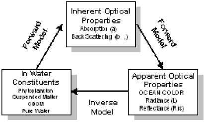
Figure 2.1 Interpretation Method of Ocean Color
Signal
Computation of Water Leaving Radiance
Normalized of water leaving radiance is defined
as:
[ Lw (—)] n = F 0(λ)[pwλn (1)
π
Where, Fo is extra terrestrial solar irradiance
(Thuillier et. al 2002). The relationship between
normalized of water leaving reflectance and
b —) = bbW —)+bbc —, chl)+⅛s —, SS) (8)
Water bbw(λ) (Smith and Beker, 1981), Chlorophyll-a bbc(λ) (Mobly, 1994)
bbc —) = 0.0087× bc (—)
remote sensing reflectance is
[ρw(—)]n = π(t / n)2 Rrs(—)
bc (λ) = 0.27 × chl0.698
(2)
550 3 λ J
-0.2983
(10)
Where, t is transmittance of upward radiance and
downward irradiance across the sea surface. n is refractive index of salt water (t/n)2 value is 0.544 (Austin, 1974). Rrs is related reflectance (R) that is ratio of upward and downward irradiance (Lee, et.al 1994).
Rrs (λ) = 0.533R (λ)/ Q
Q is irradiance radiance ratio. Q = 4.5
R(λ) can be expressed as (Joseph, 1950)
k(—) - a (—)
R (—) —
k (—) + a (—)
(4)
Where k(λ) is attenuation coefficient, function of
total absorption a(λ) and backscattering
coefficient bb(λ).
k (λ) — ^ a (λ)[ a (λ) + 2.0 bb (—)]
(5)
a(λ) is contributed by water aw(λ) (Pope and Fry, 1997), chlorophyll-a ac(λ) proportional with
concentration and CDOM ay(λ).
a (—) = aw, (—) + ac — chl) + ay (λ, ay (440)) (6) ay(λ).can be expressed as (Bricaud et.al, 1983)
ay (—) — ay (440) ■ exp{- 0.014 ■ (— - 440)} (7)
bb(λ). is sum of backscattering coefficient
and suspended matter bbs(λ) (Fischer and
Kronfeld, 1986)
bbs (—) = bs (λ) ■ 0.01478
bs (—) = 0.125 ■ SS ■
—) 550 J
-0.812
(12)
With concentrations range in log scale from 0.001-
64 μg∕l of chlorophyll-a, 0.01-50 mg/l of suspended matter, and CDOM absorption at 440nm of 0.001-5 m-1 and wavelength (λ) 412, 443, 488, 531, 551 nm mixture of concentration are made by constellation of 110.592 data set of normalized water leaving radiance, constructively by FORTRAN.
Neural Network Simulation
The Artificial Neural Network (ANN) adopted the feed-forward back propagation model, which was good for the optimization and computation. The feed-forward model consists of input layers, output layers and one or some hidden layers between them. Each layer consists of several neurons, and each neuron is linked to neurons in neighborhood layers with different
weights and biases. The information from input layers is feed-forwarded through processing neurons in hidden layer to the output neurons. The
output value O of each neuron is calculated by:
O = S(- bias + x w )
i i (13)
where, bias is a specific value for each ‘neuron’, Xi is output value of neuron in the former layer, Wi is the weight of incoming-link, S is the
Sigmoid tangential function as follows:
s (x) =
1 - exp(-2 x)
1 + exp(-2 x)
(14)
where, x is the activation value (i.e. the scalar product of the synaptic weight and input vector). The ANN was trained by the error back
propagation procedure to adjust the biases and the weights of link. By using the ‘training set’, the ANN training is repeated until the mean squared error (MSE) being minimum. The MSE is defined as follows:
MSE = -Y (NNoutv ut - trueval output value
n output
(15)
Simulation is do by preparations phase and operations phase.
Preparations of Simulation
The data sets is separated randomly uniform distribution for two data sets, i.e. training sets (88.474) for teaching, and test set (22.118) for validation during the ANN training. All parameters are rescaled into a [-1, 1] amplitude before training the neural networks. Bias and weight is generated randomly balance. Inputs are
normalized water leaving radiance, output are concentration of water constituents.
Operation of Simulation
Each of these sets was then applied to the MatLab. The following network specific parameters were used: Learning function Gradient descent with momentum. Learning rate: 0.2 momentums: 0.8. Training function was used according to Levenberg-Marquardt optimization. Network training will stop by stopping procedure after a given MSE: 0.001.
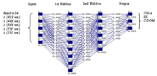
Figure 2.2 Artificial Neural Network
Field Observation Data
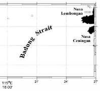
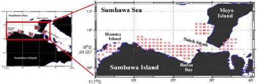
The measurement distribution of
Chlorophyll-a and turbidity concentration at Badung Strait Bali W115.05 E115.63 N-8.41 S-8.89 (59 points) and north coast of Sumbawa island W115.05 E115.63 N-8.0 S-8.89 (152 points) is done on May 2-12, September 5-9, and November 14-18 2005. The north coast of
Sumbawa island observation is included in this
study in case of getting good validation. Bali
island and Sumbawa island has similar latitude. Equipments for water quality check are WQC-22A/24 TOA-DK and Compact-CTD ACTD 650/687 Alec electronic. In-situ data are used to validation of ANN simulation results.
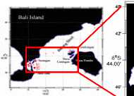
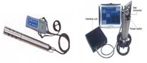
Figure 2.3 (a) Water quality check WQC-24 TOA-DK and (b) Compact-CTD ACTD 687 Alec electronic
(
Figure 2.4 Stations of Sampling Data (a) Bali (b) Sumbawa
Satellite Data
MODIS (Moderate Resolution Imaging Spectrometer) satellite data with radiometric calibrated and geolocated radiances L1B 1km swath data are use for application. Date of acquisitions is synchronous with date of field observation. Satellite data is processed to level-2
products by SeaDas software. Atmosphere corrections are selected of four algorithms to get minimum negative water leaving radiance. The models are, (a).Multi-scattering fix model coastal 70% humidity, (b).Multi-scattering with 765/865 nm model, (c).Multi-scattering with 765/865 nm and NIR 10 time iteration, (d).Multi-scattering with 765/865 nm and NIR 50 time iteration. Products are normalized water leaving radiance which as input to ANN. Also, OC3M for chlorophyll-a product provide by NASA standard algorithm is used for comparison with in-situ data.
RESULT AND DISCUSSION
Computation of water leaving radiance is
giving unique characteristic curve of absorption,
backscattering and normalized water leaving
radiance (Lw)N with separately concentration of
three water constituents.
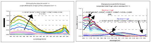
Figure 3.1 Curve characteristic of chlorophyll-a (a) Absorption (b) Radiance
Chlorophyll has two peak absorption (figure 3.1 a), fist is pigment peak at 440 nm (50 µg/l ∼ 2.01 m-1) and second is fluorescent peak at 665 nm (50 µg/l ∼ 0.945 m-1). Radiance has two type curve (figure 3.1b), less concentration than 1.0 µg/l and equal and greater concentration than 1.0 µg/l. Curve characteristic cross at 530 nm.
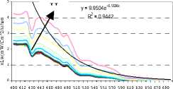
Figure 3.2 showed radiance curve characteristic of suspended matter and CDOM with various concentration. Both has similar characteristic, energy is exponentially decreasing toward longer wavelength.
Suspended Matter nLw(mW/Cm^2/sr/um) (Chlorophyll-a 0.1 mg/m^3 yellow substance 0 m^-1)
wavelength(nm)
Yellow Substance nLw(mW/Cm^2/sr/um) (Chlorophyll-a 0.1 mg/m^3 suspended matter 0 mg/L )
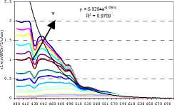
wavelength(nm)
Figure 3.2 Radiance Curve characteristic of (a) Suspended matter (b) CDOM
ANN training has 259 epochs and MSE is 0.000999505. Test is giving good correlation result. Coefficient determination (R2) for test of all substance is above 0.81 (Figure 3.3a-c). This network is valid for simulation
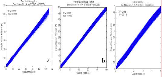
Figure 3.3 ANN test results. (a) Chlorophyll-a (b) Suspended matter (c) CDOM
Field observation result for distribution of chlorophyll-a and turbidity are showed in contour map (Figure 3.4a-d). At Badung Strait Bali
Chlorophyll with range 0.01-35.1µg/l, turbidity with range 0.1-7.7 mg/l. At North Coast of Sumbawa Chlorophyll with range 0.01-36.51µg/l, turbidity with range 0.00-13.84mg/l. Measurement
at surface layer (less than 1 m).
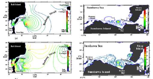
Figure 3.4 Distribution of chlorophyll-a (a), turbidity (b) Bali and Sumbawa (c-d).
Selection of atmosphere correction gives algorithm-d is less negative water leaving radiance (6.77% pixels). Algorithm-c gives 6.80% pixels of negative Lw (figure 3.5a), but gives 44 second faster than algorithm-d (figure 3.5b).
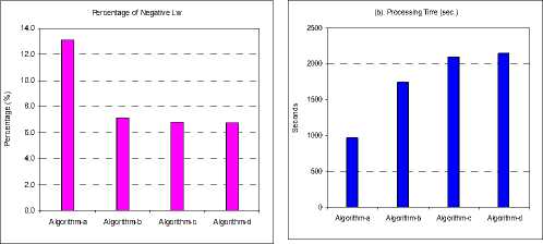
Figure 3.5 Percentages of nLw (a) and Processing Times (b) of Algorithms
Estimate concentration for chlorophyll-a, minimum is 0.001 maximum is 35.10 µg/l. For suspended matter, estimate concentration
minimum is 0.01 maximum is 7.7 mg/l. For
CDOM, estimate concentration minimum is 0.001
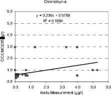
by NASA as standard algorithm gives R2 0.1884 with RMS is 1.325 µg/l.
maximum is 5.0 mg/l. Distribution concentrations
in detail are shown in figure 3.6.
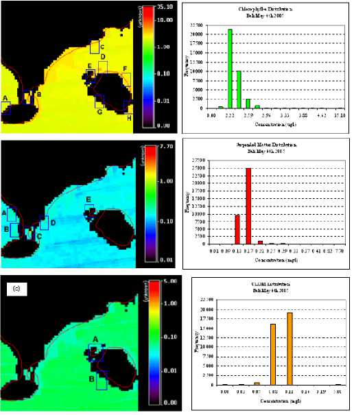
Figure 3.6 Distributions of Chlorophyll-a (a),
Suspended matter (b) and CDOM (c)
from inverse model at Bali area May 4th 2005
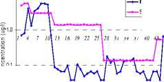
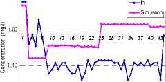
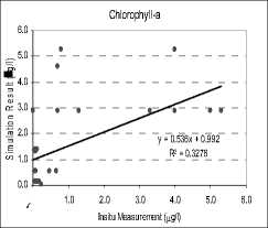
Only 49 (23.22 %) data are selected can be use for validation, because cloud coverage on site and lack of satellite data. Comparison between in-situ and simulation result is giving R2 0.3276 for chlorophyll and 0.4086 for turbidity. No in-situ measurement for CDOM For chlorophyll-a RMS is 1.473 µg/l, for suspended matter RMS is 1.319 mg/l. Comparison with another study is used OC3M chlorophyll-a empirical algorithm provide
Chlorophyll-a in-situ vs. simulation
10.0
Simulation
1.0
31 34 37 40
0.1
Position (St.)
10.00
In-situ
Turbidity in-situ vs. simulation
1.00
0.10
0.01
Position (St.)
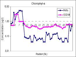
Figure 3.8 Comparison between in-situ and OC3M chlorophyll-a
Less accuracy of validation causes by some reasons. Like measurement technique, atmosphere condition and synchronized acquisitions between measurement and satellite images, so getting match-ups data is difficult on site. Those are main problem in passive ocean color. Output simulation is higher compared with in-situ data. In-situ data is
In-situ
Simulation
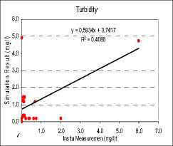
Figure 3.7 Comparison between in-situ and simulation (a) chlorophyll (b) suspended matter
more varies and fluctuation compared with output simulation. The reason is due to concentration of substance (chlorophyll-a, suspended matter) obtained from satellite data is not just for surface value, actually it is an average effect in light penetrating zone. Atmosphere condition, like thin cloud and present of aerosol are also influence of magnitude of radiance which detect by sensor become high, therefore chlorophyll-a concentration obtained from satellite higher than in-situ data. Another reason is difference method used to detect concentration of the substance between satellite and in-situ measurement. This study used radiance reflected method as phytoplankton pigment to detect concentration of the substance, while in-situ measurement for chlorophyll-a used fluorescence line height method. Construct the vertical profile distribution pattern chlorophyll-a with considering the light penetrating in the site research location, develop validation protocol by use HPLC (high performance liquid Chromatography) analysis to measure chlorophyll-a concentration and gravimetric to inorganic suspended matter, improved of atmosphere correction algorithm are important to be carried out for accuracy of validating results. Reason about in-situ data more varying and fluctuation compared with output simulation, because transect of the stations doesn’t agree with spatial resolution of the satellite data, where minimum distance for each stations must
more than 1 km. One pixel (1.000 m2) has same concentration of substance.
CONCLUSION
In this study, it is described that, multiscattering with 765/865 nm and NIR 10 time iteration is the best selection for reduce negative water leaving radiance in case of coastal around Indonesia. Back propagation artificial neural network has ability to solve inverse problem with three unknown water constituent such as chlorophyll-a, suspended matter and colored dissolved organic matter (CDOM), from five normalized water leaving radiance in the visible bands. From case-1 oligothropic to case-2 turbid water. Back propagation artificial neural network needs training process before applied to the satellite data. OC3M empirical algorithm as NASA standard algorithm for chlorophyll-a with in-situ data gives R2 0.1884, this study gives better accuracy with R2 0.327. How ever, both studies are still giving over estimate concentration.
ACKNOWLEDGMENT
The author would like to thank and appreciate to Mr. Ohgane, Mr. Tani and Mr. Yamagata (Kyowa Concrete Ltd. Japan) for chance to get experience in oceanography observation and also for staff in MarineTech Bali for cooperation.
REFERENCES
Campbell, J.B.1987. Introduction to Remote Sensing. (Text Book) The Guilford Press 200 Park Avenue South, New York
Carder K.L, Chen R.F, Lee Z, and Hawes S.K,1999. ATBD 19 MODIS Ocean Science Team: Case-2 Chlorophyll a Version 5 Marine Science Department University of South Florida (Report) 140 Seventh Avenue South St. Petersburg, Florida 33701
Cracknell, A. and Hayes, L. 1991. Introduction to Remote Sensing. (Text Book) Taylor and Francis Ltd. 4 John St, London.
Doerffer, R. and Schiller, H, 1997. ATBD 2.12 MERIS ESL, Pigment index, sediment and gelbstoff retrival from directional water leaving radiance reflectances using inverse modeling technique, (Report) GKSS Research Center 21502 Geesthacht, Germany
Fausett, L. 1994.Fundamenal of Neural Networks (Architectures, Algorithms, and Applications). (Text Book) New Jersey: Prentice Hall.1994
Gordon, H. R. And Morel A.. 1983. Remote assessment of ocean color for interpretation of satellite visible imagery. A review. Lecture Notes on Coastal and Estuarine Study, (Lecture Notes) Vol. 4, Springer Verlag.
Hu, C., Carder, K. L. and Müller-Karger, F. E. 2000. Atmospheric correction of SeaWiFS imagery over turbid coastal waters: a practical method. (Journal) Journal of Remote Sensing and Environment. 74: 195-206.
Hung S.L., Andrew Y.S.Cheng, V, Lee C.S., 1992. Neural Network for Satellite Imageries,
Department of Computer Scince. City Polytechnic of Hong Kong SPIE. Vol.1 1992 (Journal).
IOCCG Reports 2000: Report Number 3, 2000.Remote Sensing of Ocean Colour in Coastal, and Other Optically-Complex Waters .Bedford Institute of Oceanography, (Report) Canada.
Jerlov, N. G.,1976. Marine Optics, Elsevier, (Text Book) Amsterdam, 231 p
Martin, S. 1985. An Introduction to Ocean Remote Sensing, (Text Book) Cambridge
University Press.
Osawa, T., Zhao, C., Suwa, J., 2002. Primary Porductivity Model Base on Neural Network, (Proceeding) Porsec 2002.Vol.1
Parslow, J. S, Hoepffner, N. R. Doerffer, J. W. Campbell, P. Schlittenhardt, S. Sathyendranath, 2000. Case-2 OceanColour Applications. IOCCG Reports 2000: (Report) Number 3, 2000.
Sathyendranath, S, 2000.Remote Sensing of Ocean Colour in Coastal, and Other Optically-Complex Waters. (Report) Number 3 IOCCG Reports 2000.
Toratani, M, Tanaka, A., Fukushima, H. and Kobayashi,H. 2000. Atmospheric correction scheme for turbid case II waters and its application to East China Sea OCTS data,(Proceedings) Porsec 2000.vol.1
Tanaka, A., Oishi, T., Kishino, M. and Doerffer, R. 1998. Application of the neural network to OCTS data. In: Proceedings, Ocean Optics XIV, S. G. Ackleson and J. Campbell (eds.), Office of Naval Research, (Proceedings) Washington, DC.
ECOTROPHIC | VOLUME 1 NO. 2 NOVEMBER 2006
9
Discussion and feedback