THE INFLUENCE OF LOCAL TRAFFIC ON NOISE LEVEL (CASE STUDY: BYPASS NGURAH RAI AND SUNSET ROAD, BALI)

THE INFLUENCE OF LOCAL TRAFFIC ON NOISE LEVEL (CASE STUDY: BYPASS NGURAH RAI AND SUNSET ROAD, BALI)

D.M Priyantha Wedagama¹⁾*

• ¹⁾    Department of Civil Engineering, Faculty of Engineering, Udayana University Kampus Bukit Jimbaran-Badung, Bali 80361

*Email : [email protected]

Abstrak

Studi ini meneliti pengaruh faktor-faktor lalu lintas lokal terhadap tingkat kebisingan di jalan arteri di Bali dengan studi kasus jalan Bypass I Gusti Ngurah Rai dan Sunset Road. Model regresi sederhana dan regresi berganda disusun dengan variabel-variabel volume dan kecepatan lalu lintas serta nilai kebisingan yang diperoleh dari hasil pengukuran tingkat kebisingan di kedua jalan arteri tersebut. Model yang disusun terdiri dari 1 variabel tidak bebas dan 8 variabel bebas menggunakan perangkat lunak SPSS versi 15. Hasil studi ini menyimpulkan bahwa volume lalu lintas dari sepeda motor dan jarak pengamatan kebisingan dari garis tengah jalan terdekat sangat berpengaruh terhadap tingkat kebisingan. Volume sepeda motor berpengaruh sebesar 26.7% terhadap tingkat kebisingan dan gabungan volume sepeda motor dan jarak pengamatan kebisingan dari garis tengah jalan terdekat berpengaruh sebesar 46.9% terhadap tingkat kebisingan. Semakin besar volume lalu lintas dari sepeda motor semakin tinggi pula tingkat kebisingan. Kebijakan di bidang transportasi seperti pengurangan jumlah sepeda motor di jalan raya dan pada saat yang bersamaan memperbaiki kualitas angkutan umum merupakan alternatif untuk mengurangi tingkat kebisingan. Penelitian ini juga menyarankan suatu studi lanjutan untuk menentukan jarak pengamatan yang ideal dari garis tengah jalan pada saat pengukuran tingkat kebisingan di jalan.

Kata kunci: Model kebisingan, jalan arteri, volume lalu lintas, jarak pengamatan

in developing countries. In the US and the UK for instance, the exhaust pipes of semi-trailer trucks are located on the top of vehicle cabs. In contrast, the exhaust pipe of trucks in developing countries is normally situated about 0.5 m above the ground (Pamanikabud and Vivitjinda, 2002).

• • The proportion of motorcycles in developing countries is much higher than that in developed countries.

Meanwhile, an average annual growth rate of motor vehicles in Bali is approximately 11% with the registered motorcycles annually are almost 85% of total vehicles. In 2010 there were 1,449,279 motorcycles in Bali among the 1,715,675 total vehicles registered. In the capital city of Denpasar, the number of registered motorcycles in 2010 was 477,023 of the total of 599,551 registered vehicles. During the daytime on weekdays, number of vehicles would be doubled about 900,000 units considering commuters

and students trips to and from Denpasar (Statistics of Bali Province, 2011).

There are three main modes in Bali consisting private cars, heavy vehicles (bus and truck) and motorcycles which share together the roadways including on arterial roads. Commuters use the arterial roads, which connects the capital city and the surrounding areas. Consequently, all these roads passed daily high traffic flows on which approximately 70% of the road users ride a motorcycle for their trips. This traffic condition on arterial roads in Bali certainly generated significant traffic noise on the adjacent environment in particular during peak hours.

Having considered these facts, traffic noise models originated from developed countries are not suitable to use in developing countries including Bali. Traffic noise model based on local traffic characteristics in developing countries however, are remain underdeveloped (Pamanikabud and Vivitjinda, 2002). This study therefore, is aimed at developing the traffic noise model for arterial roads in Bali using Bypass Ngurah Rai and Sunset Road as the case studies. The proposed model is based on local traffic characteristics and vehicle types using noise level measures based on a noise level measurement technique. Thus, the model is used to analyse the influence of local traffic characteristics on noise level on these two arterial roads.

highway traffic noise model consisted traffic noise levels, traffic volumes by vehicle types, average spot speeds by vehicle types and the geometric of highway sections. The basic noise level for each type of vehicles was constructed considering the direct measurement of Leq (10 seconds) from the actual running condition of each type of vehicles.

A study by Filho et.al (2004) was carried out to analyse the relationship between traffic composition and noise generated by typical Brazilian roads. Traffic composition is described as the proportion of heavy vehicles in the total number of vehicles. Data were collected from Monday to Friday from 6:00 to 10:10 a.m. A total of 149 measurements were made on three roads. Measurements were made for each the percentile level L₁₀ and the equivalent level Leq. These levels were plotted against the traffic composition and empirical expressions were obtained with sufficiently good correlation indexes.

A previous study was conducted by Watts (2005) in England to develop traffic noise model. This began due to demands on the production of strategic noise maps and noise action plans for major roads. The maps will have to be produced using harmonised prediction methods. The study was to develop the road source model, propagation models and an engineering model for use in noise mapping. Data was collected at 13 sites to validate the model that had been developed.

A traffic noise model based on the traffic conditions of Iranian cities has also been developed by Golmohammadi et.al (2009). Noise levels and other variables have been measured in 282 samples to develop a statistical regression model based on A-weighted equivalent noise level for Iranian road conditions. The results revealed that the average LAeq in all stations was 69.04± 4.25 dB(A), the average speed of vehicles was 44.57±11.46 km/hour and average traffic load was 1231.9 ± 910.2 vehicles/ hour. The developed model has seven explanatory entrance variables in order to achieve a high regression coefficient (R²=0.901).

Two recent studies were carried out by Baskoro (2011) and Jayanti (2011) using bypass I Gusti Ngurah Rai and Sunset Road as the case study area. These studies determined noise equivalent number for each type of vehicle consisting motorcycle, light and heavy vehicles. A study by Jayanti (2011) found that noise equivalent numbers for motorcycle, light and heavy vehicles are 0.375, 1 and 8.125 respectively.

Meanwhile, a study by Baskoro (2011) concluded that noise equivalent numbers for motorcycle, light and heavy vehicles are 0.571, 1 and 13.5 respectively. These equivalent numbers are then used in this study to determine the environment passenger car units (enpcu) as described in model development section.

• 3.    Research Method

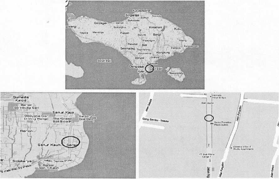
  • 3.1    Case Study Area and Data Collection Bypass Ngurah Rai connects between Tohpati and Nusa Dua spanning about 30 km and has been in operations since 1981. Meanwhile, Sunset Road is linking between Kerobokan and Kuta in Badung regency. Both bypass I Gusti Ngurah Rai and Sunset Road are a dual carriageway which has a median. These two arterial roads provide access into many tourist destinations including Kerobokan, Kuta, Sanur, Nusa Dua, Uluwatu and Jimbaran. As the results, thousands of vehicles everyday pass on these roads. Figures 1a and 1b depicts the location of bypass I Gusti Ngurah Rai and Sunset Road.

    

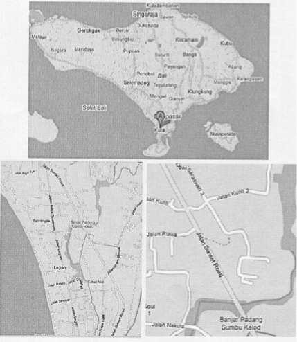
    Figure 1a. Case Study Area- Sunset Road Traffic data including vehicle speed, traffic

    
    
    
    
    

Figure 1b. Case Study Area-Bypass Ngurah Rai

volume and noise data are collected on road links where:

• •    no junction and traffic lights are located nearby which possibly decreasing the speed of vehicle movement.

• •    no noise sources other than the traffic.

• •    no high wall or high buidling are located nearby

which possibly reproduce noise on the Sound Level Meter device.

The survey location for both arterial roads are circled on Figures 1a and 1b. Data collection on Sunset Road and bypass I Gusti Ngurah Rai are carried out from 8am to 7pm on 25 Januari 2011 and 1 Februari 2011 respectively.

As shown in Figure 2, the Sound Level Meter (Receiver P) is placed upon a tripod so that the microphone position is 1.2 m high from the ground and a certain distance from the road edge and road centre lines (D_n and D_f). The microphone is exposed with an upright position to noise source. Noise and traffic data are recorded and measured at intervals of

15 minutes. This is because in highly mixed traffic on roadways, it is always wise to observe these measures cautiously at short period counts (O’Flaherty, 2005).

Traffic volumes are classified according to the direction and type of vehicles. Speed data collection is taken at interval of 900 seconds (15 minutes) for a one-time observation or for one sample and is recorded along with the time measurement of noise level and traffic volume. Speed data is collected using two marker lines for a length of 50 meters. Observers using a stopwatch record the time at which the vehicle crossing the line from the first marker to the second marker.

The number of motorcycles on bypass I Gustri Ngurah Rai are accounted for by 55% of total vehicles and are about 5000 motorcycles per hour during peak hour. Meanwhile, during peak hour the number of motorcycles are accounted for by 72% of total vehicles and are about 4000 motorcycles per hour on Sunset Road.

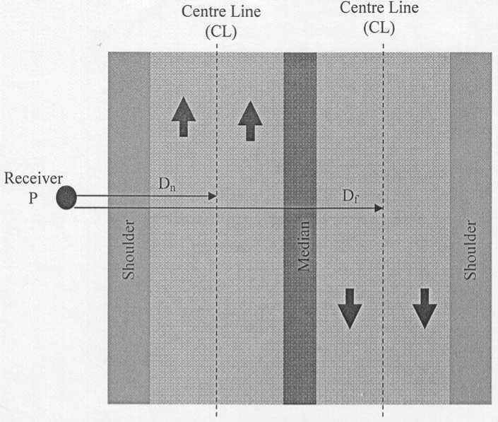
Figure 2 Noise Measurement on an Arterial Road

• 3.2 . Model Development

A dependent and eight independent variables are employed in this study. Equivalent noise level in units of dB on an A weighted scale (dBA) is used as a dependent variable. Equivalent noise level (Leq) is defined as the constant noise level consisting the same quantity of acoustical energy as the real fluctuating level of interest over the same period of time. Meanwhile, space mean speed of vehicles is defined as the average speeds over a length of roadway.

Each type of vehicle (i.e motorcycle, light and heavy vehicles) produces noise level differently depending on their size and engine size so that a coefficient is required to standardise that noise level. This coefficient is defined as environmental passenger car units (enpcu). The enpcu of the total traffic volumes for each type of vehicle were obtained from two previous studies for the same case study area (refer to Jayanti, 2011 and Baskoro, 2011). The noise and traffic volumes data used for this study are shown in Tables 1a and 1b.

Table 1a. Noise and Traffic Volumes data in Bypass Ngurah Rai

Time Measurement	Qmc	Qlv	Qhv	Leq (dBA)	Time Measurement	Qmc	Qlv	Qhv	Leq (dBA)
07.00-07.15	493	403	13	70.82	13.00-13.15	547	452	17	72.63
07.15-07.30	555	406	10	71.43	13.15-13.30	572	460	15	73.77
07.30-07.45	477	380	17	70.15	13.30-13.45	567	493	19	75.12
07.45-08.00	493	410	16	72.36	13.45-14.00	594	493	22	75.08
08.00-08.15	560	515	17	73.10	14.00-14.15	678	514	26	75.44
08.15-08.30	683	539	20	72.81	14.15-14.30	717	549	27	76.86
08.30-08.45	636	540	21	73.11	14.30-14.45	741	528	24	-J7726-
08.45-09.00	641	512	19	72.92    -	14.45-15.00	783	533	26	78.75
09.00-09.15	544	520	11	73.29	15.00-15.15	808	551	27	80.06
09.15-09.30	498	481	15	74.14	15.15-15.30	802	534	14	83.76
09.30-09.45	504	452	19	72.82	15.30-15.45	808	523	19	87.03
09.45-10.00	518	509	14	72.97	15.45-16.00	812	515	30	91.35
10.00-10.15	532	479	15	72.51	16.00-16.15	827	524	13	95.77
10.15-10.30	530	505	14	72.32	16.15-16.30	836	513	17	97.81
10.30-10.45	523	468	16	72.15	16.30-16.45	847	531	19	102.29
10.45-11.00	497	506	13	71.77	16.45-17.00	810	506	17	104.40
11.00-11.15	554	493	13	71.52	17.00-17.15	763	484	15	99.60
11.15-11.30	658	467	21	71.49	17.15-17.30	672	472	20	72.96
11.30-11.45	578	482	15	72.10	17.30-17.45	556	435	10	71.05
11.45-12.00	698	496	25	71.00	17.45-18.00	539	425	10	71.22
12.00-12.15	490	448	14	71.29
12.15-12.30	495	385	15	71.19
12.30-12.45	582	476	12	71.72
12.45-13.00	613	532	15	72.77

Note:
(Leq)	Equivalent noise level (dBA)
Qmc	Traffic volume of motorcycle (vehicles)
Qlv	Traffic volume of light vehicle (vehicles)
Qhv	Traffic volume of heavy vehicle (vehicles)

Table 1b. Noise and Traffic Volumes data in Sunset Road

Time Measurement	Qmc	Qlv	Qhv	Leq (dBA) :	Time Measurement	Qmc	Qlv	Qhv	Leq (dBA)
08.30 - 08.45	1127	364	26	72.30 ⅛	13.00-13.15	813	402	28	71.46
08.45 -09.00	1251	300	20	71.98 ? i	13.15 - 13.30	831	390	27	71.90
09.15 -09.30	1339	397	26	72.5o : ;	13.30-13.45	951	408	25	71.76
09.45 - 10.00	992	387	24	72.45 L	13.45 - 14.00	924	434	30	71.89
10.00- 10.15	803	445	21	71.37	14.00- 14.15	1003	431	33	73.13
10.15-10.30	825	367	23	71.84	14.15-14.30	978	388	25	72.08
10.30-10.45	950	423	24	71.94	14.30-14.45	1006	410	24	72.11
10.45-11.00	936	447	25	72.03	14.45-15.00	1156	430	25	72.26
11.00-11.15	1002	421	27	72.82	15.00-15.15	1174	445	27	72.61
11.15-11.30	1003	405	22	72.23	15.15- 15.30	1178	437	27	73.14
11.30-11.45	942	411	29	72.12	15.30-15.45	1234	465	31	73.15
11.45-12.00	1139	416	27	72.17 >	15.45 - 16.00	982	348	19	70.97
12.00-12.15	951	444	27	72.75	17.15-17.30	1445	386	31	73.02
12.15-12.30	1082	442	30	73.13	17.30-17.45	1433	374	30	72.91
12.30- 12.45	880	434	24	72.15	17.45- 18.00	1103	395	23	71.68
12.45-13.00	897	392	26	72.32      ■	18.45-19.00	807	306	19	70.27

Note:

(Leq) : Equivalent noise level (dBA)

Q_mc : Traffic volume of motorcycle (vehicles)

Q_lv     :   Traffic volume of light vehicle (vehicles)

Qhv     ∙   Trafficvolumeofheavyvehicle(Vehicles)

All dependent and independent variables are regression models using the statistical software of shown in Table 2. All variables are then employed to SPSS version 15.

develop the simple regression and multiple

Table 2. Study Variables

Dependent variable

Y : (Leq) Equivalent noise level (dBA)

Independent variables

Q_MC :   Total traffic volume of motorcycle (enpcu/hour)

Q_LV :   Total traffic volume of light vehicle (enpcu/hour)

Q_HV :   Total traffic volume of heavy vehicle (enpcu/hour)

V_MC : Space mean speed of motorcycle (km/hour)

V_LV : Space mean speed of light vehicle (km/hour)

V_HV :   Space mean speed of heavy vehicle (km/hour)

D_n :   Distance from observation point to the nearest road centre line (m)

D_f :   Distance from observation point to the farthest road centre line (m)

• 4.    Results and Discussions

Simple regression models, which using one significant independent variable, are developed. The selected model must have its significance less than or equal to 5% and the determination coefficient (R²) is close to 1. As shown in Table 3, a significant variable which considerably influencing noise level is determined. Having compared to light and heavy vehicles traffic volume and observation distances, motorcycle traffic volume has the strongest relationship to noise level on bypass I Gusti Ngurah Rai and Sunset Road. Based on the R² value, motorcycle traffic volume influenced about 26.7% of noise level on these two arterial roads.

Table 3. Simple Regression Models

No	Model	Model Significance	R2
1.	Y= 53.93+0.057QMC	0.000	26.7
2.	Y= 48.74+0.058QLV	0.000	20.8
3.	Y= 67.82+0.032QHV	0.038	5.7
4.	Y= 82.26-0.931Dn	0.004	10.7
5.	Y= 113.49-2.597Df	0.004	10.7

As mentioned previously, in a simple regression model simply considers the relationship between one predictor (independent variable) and dependent variable. In order to analyse the relationship between several local traffic variables and noise level at once however, multiple regressions are developed. In this study, multiple regression models are constructed using stepwise method. The best model is selected on the assumption that:

• a.    the determination coefficient (R²) is close to 1. b. the significance value of ANOVA test is less

than or equal to 5% and each independent variable must have a significance value less than or equal to 5%.

• c.    no correlation is found between independent variables within the model.

• d.    either the sign of + or – of each independent variable is logically accepted.

Table 4 shows two models obtained using the stepwise method. Motorcycle traffic volume and observation distance influenced about 46.9% of noise level on these two arterial roads. In other words, 46.9% of the variability in noise level can be explained by motorcycle traffic volume and observation distance while the remaining 53.1% is due to other unexplained factors. The model therefore, could probably benefit from the inclusion of other variables.

In addition, the large model constant indicates that there will be some other factors, for instance interaction between tyres and road surface, road conditions (e.g. pavement conditions) and car horn blown related factors that may be impacted on noise level on these two arterial roads. It is suggested therefore, to further develop the noise model which include these variables.

From the two models (i.e. the simple and multiple regression models) suggested that the larger motorcycle traffic volume the higher noise level. It is therefore, transport policies such as limiting the number of motorcycle while at the same time upgrading the public transport may be considered to decrease noise level. In addition, it is suggested that the farther observation point to the nearest road centre line the lower noise level. In this study, the observation distance to the nearest centre line is 5.5m. Further study however, is required to determine an appropriate observation distance on noise level measurement.

• 5.    Conclusions

Both single and multiple regression models are developed to investigate the influence of local traffic characteristics on noise level. Two significant variables influencing noise levels are motorcycle traffic volume and observation distance to the nearest road centre line. Motorcycle traffic volume influenced

Table 4. Multiple Regression Models

No	Model	Model Significance	R2
1.	Y= 104.018+0.068QMC -3.362 Df	0.000	46.9
2.	Y=59.976+0.068 QMC-1.313Dn	0.000	46.9

about 26.7% on noise level and both motorcycle traffic volume and observation distance to the nearest road centre line influenced about 46.9% on noise level. In addition, the large model constant however, indicates that there will be some other factors, for instance interaction between tyres and road surface and car horn blown related factors that may be impacted on noise level on these two arterial roads.

This study suggested that the larger motorcycle traffic volume the higher noise level. It is therefore, transport policies such as limiting the number of

motorcycle while at the same time upgrading the public transport may be considered to decrease noise level. In addition, it is suggested that the farther observation point to the nearest road centre line the lower noise level. Further study however, is required to include some other variables consisting interaction between tyres and road surface, road conditions (e.g. pavement conditions), car horn blown related factors determine and an appropriate observation distance on noise level measurement.

References

Baskoro, W.S.A. 2011. Modelling on Vehicle Noise on Sub Urban Arterial Road Link with Median (Case Study: Bypass Ngurah Rai). (In Indonesian). Final Project. Departement of Civil Engineering Faculty of Engineering Udayana University, Denpasar.

Filho, J.M.A., A. Lenzi, and P.H. Zannin. 2004. “Effects of Traffic Composition on Road Noise: A Case Study”. Transportation Research Part D, 9. 75-80.

Golmohammadi, R., M. Abbaspour, P. Nassiri, and P. Mahjub. 2009. “A Compact Model for Predicting Road Tracffic Noise”. Iran. J. Environ. Health. Sci. Eng., 6.3.181-186.

Jayanti, M. 2011. The Analysis of Vehicle Noise Equivalent on Traffic (Case Study: Sunset Road, Badung Regency). (In Indonesian). Final Project. Departement of Civil Engineering Faculty of Engineering Udayana University, Denpasar.

O’Flaherty, C.A. (Ed). 2005. Transport Planning and Traffic Engineering. Elsevier Butterworth-Heinemann. Oxford.

Pamanikabud, P. and P. Vivitjinda. 2002. “Noise Prediction for Highways in Thailand”. Transportation Research Part D, 7. 441-449.

Setiawan, R., T.D. Arief., N. Handayani, and P. Sawitri. 2002. Tollway Noise Modelling: Waru-Sidoarjo. (In Indonesian). Petra Christian University, Surabaya.

Statistics of Bali Province. 2011. Bali in Figures. (In Indonesian). Denpasar.

Watts, G.R. 2005. Harmonoise Production Model for Road Traffic Noise. Transport Research Laboratory. England.

31