STUDY OF AIR-SEA INTERACTION AND CO2 EXCHANGE PROCESS BETWEEN THE ATMOSPHERE AND OCEAN USING ALOS/PALSAR (Study Cases of Wind Wave Bubbling Process in Badung and Lombok Straits)

Studyofair-Seainteractionand co₂ exchange process between Theatmosphereand ocean usingalos/palsar (Study Cases of Wind Wave Bubbling Process in Badung and Lombok Straits)

Ni Wayan Ekayanti¹⁾, Takahiro Osawa¹⁾, I Wayan Kasa²⁾, and A. Rahman As-syakur^l)

• ^1,    Center for Remote Sensing and Ocean Science (CReSOS), Udayana University, Bali-Indonesia

• ²⁾    Master Degree Program, Study Program OfEnvironmental Science, Postgraduate Program, Udayana University, Bali-Indonesia

Abstrak

Peningkatan CO₂di atmosferyang berpotensi menghasilkanpemanasan global telah Inetjadiperhatian bagi kehidupan manusia. Lautan mengandung Iimapuluh kali lebih besar CO₂ daripada atmosfer dan men jadi penyangga yang membatasi konsentrasi CO₂ dalam atmosfer. CO₂ mengalami perubahan secara terus menerus antara udara-lautan dan konsentrasi CO₂ di dalam laut dikendalikan oleh parameterfisika, kimia, dan biologi. Perubahan konsentrasi CO₂ antara udara-lautan dapat ditentukan dari interaksi gas danperbedaan konsentrasi CO₂ antara udara-lautan. Perubahan CO₂antara udara-lautan dapat dikaji dari studi kecepatan angin, koefisien gesekan kecepatan anginyang diperoleh dari satelit ALOS/PALSAR di daerah SelatBadungdan SelatLombok, salinitas, danjuga dengan SSTyang diperoleh dari satelit MODIS.

Hasil analisis menunjukkan bahwa koefisien perubahan CO₂, perbedaan tekanan CO₂ antara udara-lautan, dan CO₂jlux antara udara-lautan secara berturut-turutyaitu 0.303±0.006 (rata-rata±standar deviasi) (mol m'² month'¹ μatm'), 17.94±10.79 iatm, and 5.35±3.26 (mol m'² month'¹), dengan nilai ^makS^{imum dan minimum dari koefisien} p^{erubahan co}2 ^{secara berturut-turut ter}j^adi p^{ada bulan}

Agustus dan Februari.

Kata kunci: CO₂, koefisien, suhu, laut.

• 1.    Introduction

Carbon dioxide (CO₂) is principal greenhouse gas (Frankignoulle et al., 1998). The direction of CO₂ gas movement depends on the CO₂ concentration gradient between air and surface water (Schimel et al., 2001). The amount of CO₂ exchange is related to the gas exchange coefficient. All water areas (Oceans, Straits, Lake, etc), with their big or small area but large atmospheric CO₂ flux are important to understand the CO₂ fluxes in continent (Meybeck, 1993). Fluxes, sources, and mechanisms of CO₂ in ocean have been previously studied and compared (Sugimori and Zhao, 1995 and Hope et al., ¹⁹⁹⁶>;.......... . .

Meanwhile, the world ocean plays an important role in the earth climate. It is not only absorbs heat from the sun, but plays a major role in carbon cycle processes (Akiyama, 2002). Ocean contains more than fifty times carbon in the atmosphere and can be taken as a buffer limiting the concentration of CO₂ in atmosphere (SugimoriandZhao, 1995). Forlongterm climate forecasts, knowledge ofthe heat, momentum,

and substance exchange between the atmosphere and the ocean is essential because the time constants and capacities of the ocean are much larger than those of the atmosphere.

Carbon dioxide (CO₂), as the main greenhouse gas in the atmosphere, has been studied for many years. An increase in the atmospheric concentration of carbon dioxide (CO₂) has been directly observed over the past 40 years in Hawaiian Island from 315 PPMV (partper million in volumes) to358 PPMV in 1994 (Keeling, 1995) and in 2004 become 380 PPMV Pre-industrial concentration at 270-280 PPMV and there is no doubt that the carbon dioxide (CO₂) concentration in the atmosphere will continue to increase in the future. Some numerical models have been developed to describe the climate response as carbon dioxide (CO₂) concentration increases, and the results show that globally average temperature on the earth surface would increase from 1.5 to 5 Celsius degree due to different model, if the carbon dioxide (CO₂) concentration will be produced to be double of the recent concentration (Keeling, 1995).

Since the growth rate of carbon dioxide (CO₂) in atmosphere is less than the rate of carbon release, some released carbon dioxide must be absorbed by either the terrestrial biosphere or the oceans.

Wind speed and wind friction velocity are not only the factor influencing the gas (CO₂) transfer ^ve∣^o⅛^y wrtolence ^wave br^eak,n^g. and bubbly are also the main factor in gas exchange (Sugimori and Zhao, 1995). The determination of wind speed and wind friction velocity from satellite-derived wind data will take an important role for air sea interaction in the ocean (Suzuki et al, 2002). Ocean wave directional spectrum is much more important parameter for describing the essential structure of ocean wave. It is generally agreed that additional wave information such as wavelength, wave direction, and perhaps wave height are contained in SyntheticAperture Radarwave image (JAXA, 2005).

PALSAR is an active microwave sensor using L-band frequency to achieve cloud-free and day-aad^-ni^ght land oration ⁽ J^axa- ZWJ) J. provides higher performance than the JERS-1 s

synthetic aperture radar (SAR). This research, study of wind wave bubbling process is located in Badung and ^L»rnbo^{k S}t™ts be^cans^e «reset areas are important places for the transportation between Ball and Lombok, and also near from land. The image data sHer.ld be lata ^{in de}e^p wato related t^o the main wavelength, so the wind wave parameters could be found easily. The Lombok strait, a small sea channel between the islands Bali and Lombok, is the second most important trans-section in southern part of the Indonesian through-flow. The aims of this research are to know the air-sea interaction at sea surface and the CO₂ exchange process between the atmosphere and the ocean using ALOS/PALSAR.

• 2.    MaterialsAnd Methods

Research Location

.   T^he ∕^esearch,l^oc^{ation are} iⁿ B^{adung and}

Lombok Straits with the geographical position is J²⁵^!^⁵^-^⁰,^^ The location of research is shown in Figure 1.

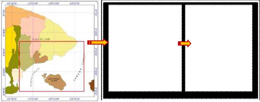
(a)                                                 (b)

Figure 1. Location OfResearch in Badung and Lombok Straits

• (a)    Location of Research and

• (b)    Directional Wind Wave Spectrum in area ofBadung and Lombok Straits after Fast Fourier Transform. Digital image of ALOS/PALSAR at January 6^th 2007.

Research Procedures

Digital image processing

The image from ALOS/PALSAR is processed in GIS software. The digital image processing is divided into three steps there were: data selection, geometric correction, and Fast Fourier Transform (FFT).

Data Calculation

• 1)  Spectral Form of Wind Wave in High Frequency

S (ω) = 2παgu *ω^-p          (1)

Spectral form of wind wave in high frequency can be expressed as follows:

Where: = Wind wave energy density, g = gravity acceleration (ms'²), u* = coefficient of friction velocity, = a constant = 0.0214, = Peak Frequency, Where, p = 1.538 to 6 (Toba and Chaen, 1973). From Equation (1) wind friction velocity (u*) is calculated.

• 2)    The estimation of Whitecap coverage (W)

The fraction of whitecap coverage due to the wave breaking has been investigated for many years such as by Monahan and Spillane (1984), T^oba ._i ^chaen (i⁹⁷³),^{and Wu} <_l9₈₈>. Generally, whitecap coverage (W) is related to the wind speed or wind friction velocity. Area ratio of whitecap on Whitecap Model can be expressed as follows: W = 0.066 U* (2)

• 3)   Carbon dioxide (CO₂) calculation

• a)    Air-sea CO₂ gas transfer velocity

Air-sea CO₂ gas transfer velocity can be calculated as follows (Monahan and ^Sp^illane,^1984):

K K (1-W) + K W         (3a)

radon m                e

Where, K = transfer velocity associated without Whitecap area = 9.58 cm/hr, K_e = transfer velocity related a turbulent Whitecap area = 475.07 cm/hr, W = area ratio of whitecap on Whitecap model, K _radon = transfer function of gas (cm/hr), Carbon dioxide gas transfer velocity can be calculated as follows:

v            ( ScCO^{2 - n}

CO2      radon ⁽Sc , )                 ^(3b)

cradon

Where: K_c02   = CO₂ gas transfer

velocity,

Sc _c02 = 2073.1 - 125.62T + 3.6276T² -4.3219x10'²T³

Sc , = 3412.8 - 224.30T + 6.7954T²-radon

8.3x10'²T³

• b)    Air-sea CO₂ gas exchange coefficient Air-sea CO₂ gas exchange coefficient calculation with equation (Akiyama, 2002):

Eco = Kco * Lco              (4)

co2      co 2    co 2

Where: = CO₂ gas exchange coefficient (cm/hr), = CO₂transfervelocitycm/hr), = CO₂ gas solubility (mol/liter atm).

• c)   Carbon dioxide (CO₂) gas solubility

Weiss (1974) provided an empirical formula to estimate CO₂ gas solubility L on the basis of data fitting between the solubility, temperature, and salinity as follows:

lnL=A1+A2(100/T_abs)+A3 ln(T_abs/100)+ S [(B1 + B2(T_abs /100) + B3(T_abs /100)²] (⁵)

Where, T_abs = absolute temperature (K) = (273.15+ T^o Celsius) K,S = salinity (psu),

• d)    Carbon dioxide (CO₂) flux calculation The carbon dioxide flux can be calculated as follows (Akiyama, 2002):

F = * (pCO_{2 t b} - pCO_{2 t} )(6)

^u 2 atmosphere ¹      2 seawater^{7v 7}

F= *ΔpCO₂

^{Where, F: CO}2 ^fluX ⁽μ^mol^/kg^), p('° .m e.^: CO₂ partial pressure in atmosphere (μatm), pCO,   , : CO, partial pressure in

• ¹    2seawater         2 ¹¹

seawater(μatm),∆ pCO₂: Carbondioxide partial pressure.

• e)    Carbon dioxide partial pressure (The ^pCO₂) distribution derived from sea surface temperature (SST)

The Δ p CO₂ is a function of temperature, total inorganic CO₂ concentration (T CO₂), alkalinity, and salinity. Metzl et al. (1995) tried to derive pCO,   from the relation

2water

with sea surface temperature (SST) in Indian Ocean. As pCO_{2 air} in the atmosphere varies slowly in both spatial and temporal scale, Zhou (1995) derived the difference ^of ^CO2par^tial p^{ressure between ai}r ^{and sea}

(⅛CO₂) from sea surface temperature. The relationship between ΔpCO₂ and SST is investigated using in situ data and MODIS data monthly in year 2007. Due to data limitation, related to summer and winter period are derived using least square fit method and the relation between Δ pCO₂ and SST can be expressed as:

∆pCO₂ = 0.0147Γ³ -0.1241f²-12.3453Γ + 115.5879 (4.8) (In summer period)

Where, T = Sea Surface Temperature (Celsius).

In this study, the average value of wind frictionvelocity (u*) is 0.00565 (Table 2). Under a continuous influence of wind, waves grow and eventually become unstable locally, the wave then break to dissipate excess energy provided by the wind (Wu, 1988). The breaking is marked by whitecaps.

The fraction of whitecap coverage due to the wave breaking has been investigated for many years (Monahan and David, ≡7±^ ^aTT^{973iwu 19883} Zhao, 1995). Generally, whitecap coverage (W) is related to the wind speed or wind friction velocity. Monahan and David (1989) used ordinary least square fitting (OLS) and robust bi weight fitting technique (RBF) to analyze the data set of Toba and Chaen (1973). By the way, Wu (1979) proposed that the whitecap coverage, W, should be related to the wind stress or wind friction velocity on the basis of theoretical analysis. Waves break after wind wave is supplied excessive energy by wind. Whitecap coverage (W), the fraction of the sea surface covered by whitecaps, is related to the energy flux from wind (Wu, 1988). However, the conclusion, whitecap coverage (W) should be proportional to the cube of wind friction velocity, seems to have been accepted by the scientific community (Wu, 1988).

In this work, some data of directional wind wave spectrum image have been taken in the inland sea, Badung and Lombok Straits. The data is digitized byFastFourier Transform in the computer. Toba and a^^andMo-ano⁹⁸⁴)^ reprocessed after friction velocity is reestimated on the basis of wind speed logarithmic profile. Finally, the result to determined the wind friction velocity in order to calculated whitecap coverage (W) by the modified whitecap model hereafter, ^w^⁶⁶,.-,+..-....,,..,.,.,¹.. area ratio of whitecap on Whitecap Model _τ boated, w = m^ ^ wholevalueofU*, W,andK . ,areshown ’    ⁷           radon’

ⁱⁿ?^bl^!5J;,

After the whitecap coverage coefficient is found, the processes are continued to find the transfer velocity of gas transfer associated without whitecap area (K_radon) withMonahanModelcalculation(K , = radon

K_m (1-W) + K_e W), from this equation the value of K , is found (K , = 9.58 cm radon                   radon

hour'¹). From the K , value, the radon

calculation processes are continued to get the CO₂ transfer velocity ( Kco₂) also follows the Monahan model calculation ScCO. _-f,

( KCO₂ = Kradon (~----)     ). Result is

Scradon

shown in Figure 6 (a).

The calculation processes are continued to get the CO₂ gas solubility (L), after the CO₂ transfer velocity is estimated. L coefficient then combine with CO₂ transfers velocity ( KCO^), so the CO₂ gas exchange coefficient ( E_co2) is estimated. The calculation processes are continued ^,o g.t ^ pCy. A^fter til.     ^pO .

^estⁱrnat^ed^, th. calculation P^^.s are continued to get CO₂ flux combining with CO₂ gas exchange coefficient

(Flux= Eco₂* ∆p∞2).

Table 5.1 Wind Friction Velocity (U*), W, and K_radon Calculation

S(ω)	ω (Hz)	π	α	g (ms-2)	p -2	u *	W=0.066 u*3	Kradon
67	0.006098	3.14	0.0214	9.8	3.72E-05	0.002	4.47E-10	9.58000021
108	0.005587	3.14	0.0214	9.8	3.12E-05	0.003	1.11E-09	9.58000052
188	0.005682	3.14	0.0214	9.8	3.23E-05	0.005	6.46E-09	9.58000301
278	0.005618	3.14	0.0214	9.8	3.16E-05	0.007	1.95E-08	9.58000908
338	0.006211	3.14	0.0214	9.8	3.86E-05	0.009	6.41 E-08	9.58002982
379	0.006173	3.14	0.0214	9.8	3.81E-05	0.011	8.70 E-08	9.58004050
293	0.005882	3.14	0.0214	9.8	3.46E-05	0.008	3.01 E-08	9.58001401
213	0.005780	3.14	0.0214	9.8	3.34E-05	0.005	1.04 E-08	9.58000485
188	0.005682	3.14	0.0214	9.8	3.23E-05	0.005	6.46 E-09	9.58000301
180	0.005848	3.14	0.0214	9.8	3.42E-05	0.005	6.74 E-09	9.58000314
257	0.006173	3.14	0.0214	9.8	3.81E-05	0.007	2.71 E-08	9.58001261
223	0.006993	3.14	0.0214	9.8	4.89E-05	0.008	3.75 E-08	9.58001744
209	0.006897	3.14	0.0214	9.8	4.76E-05	0.008	2.84 E-08	9.58001321
150	0.006897	3.14	0.0214	9.8	4.76E-05	0.005	1.05 E-08	9.58000488
93	0.006993	3.14	0.0214	9.8	4.89E-05	0.003	2.72 E-09	9.58000127
195	0.006803	3.14	0.0214	9.8	4.63E-05	0.007	2.12 E-08	9.58000988
80	0.006536	3.14	0.0214	9.8	4.27E-05	0.003	1.15 E-09	9.58000054
241	0.006061	3.14	0.0214	9.8	3.67E-05	0.007	2.00 E-08	9.58000933
105	0.007353	3.14	0.0214	9.8	5.41E-05	0.004	5.29 E-09	9.58000246
251	0.005348	3.14	0.0214	9.8	2.86E-05	0.005	1.07 E-08	9.58000497
182	0.005814	3.14	0.0214	9.8	3.38E-05	0.005	6.73 E-09	9.58000313
124	0.005814	3.14	0.0214	9.8	3.38E-05	0.003	2.13 E-09	9.58000099
114	0.007143	3.14	0.0214	9.8	5.1E-05	0.004	5.68 E-09	9.58000265
167	0.007042	3.14	0.0214	9.8	4.96E-05	0.006	1.64 E-08	9.58000764
					Average	0.006	1.78 E-08	9.58000829

• 3.    ResultAndDiscussions

SST MODIS Data Monthly Year 2007

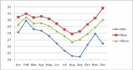
Figure 2 Graphic of annual SST value from January until December in 2007

Figure 2 shows data monthly of MODIS data year 2007 from January until December, under the temperature from 24.43⁰C to31.80⁰C. The lowest and highest temperature could be seen on August and February, with average temperature 26.69⁰C and 30.46⁰C. The minimum SST value is from 24.43⁰C in

September to 29.92⁰C in February. The maximum SST Vl” is ^fro^{m 2}≡ ^290c in Somber t₀ 3° ⁹S⁰C iⁿ February. Also, the average SST is from 26.69⁰C in August to 30.46⁰C in February. The lowest average SST is found in August and the highest is found in February 2007. Distributions of SST are shown in Figure 6 (b).

DistributionDataofMonthly ΔpCO₂ between the Atmosphere and Ocean in 2007

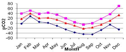
Figure3GraphicofMonthly ΔCO₂from

January until December in 2007

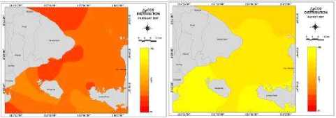
Figure 3 shows monthly data of Δ pCO₂ year 2007 from January until December, under Δ pCO₂ from -44.66 μatm to +28.78 μatm. The lowest and highest Δ pCO₂ could be seen on February and August, with average Δ pCO₂ -2.05 μatm and +39.95 μatm. The positive value of ΔpCO₂ indicates the transfer of partial pressure is from the ocean to the atmosphere which is shown in January until June and November until December during high SST in year 2007. The negative value of Δ pCO₂ indicates the transfer partial pressure is from atmosphere to the ocean which is shown in July until October during low SST in year 2007. Result shows the negative Δ pCO₂ value which indicates transfer of Δ pCO₂ into the ocean is from -22.05 μatm on August to -5.42 μatm on October. The positive Δ pCO₂ value which indicates transfer of Δ pCO₂ into the atmosphere is from 0.64 μatm on June to 39.95 μatm on February. Measurements ofthe atmospheric CO₂ concentration indicate that it has been increasing at a rate about 50% of that which is expected from all industrial CO₂ emissions(Takahashi etal., 1997).

Result also shows that the mean annual ι!∖ pCO₂ values (area weighted) for the inland sea are positive (+39.95 ± 5.21 μatm) in February, and negative (-22.05 ±9.86 μatm) in August. This means that the oceans are, as a whole, nearly in equilibrium with atmospheric CO₂, although they are locally out of equilibrium. This suggests that the oceanic uptake of CO₂ depends sensitively on the wind speed distribution where large negative ΔpCO₂ and high wind speeds prevail. The result is comparable with Takahashi climatologically data set in equator area. The result is not much different within Takahashi result. The annual mean Δ pCO₂ in this study is +34.74 μatm inFebruaryand -12.19 μatm in August. This exchange coefficient correspond Takahashi et ∙l(1997)n^s₁H÷27<>⁰^

μatm, in August (really not much different), which is global mean value ofCO₂ estimated from air-sea water equilibrium methods (Takahashi et al., 1997). Distributions of“pCO₂ are shown in Figure 6 (c).

Distribution Monthly Data of CO₂ Exchange Coefficients (The Transfer Velocity of Carbon dioxide) between the Atmosphere and Ocean in 2007

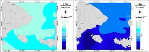
Figure 4 shows distribution monthly data of CO₂ exchange coefficients between the atmosphere and ocean in 2007 from Januaryuntil December, under

the carbon dioxide exchange coefficients from 0.27 (mol m'²month'¹ μatm'¹) to 0. (mol m'²month'¹ μatm'¹). The lowest and highest transfer velocity of carbon dioxide could be seen on February and on August, with average CO₂ exchange transfer velocity 0.28 (mol m'²month'¹μatm'¹) and 0.32 (mol m'²month'¹ μatm'¹). The CO₂ transfer velocity which is determined from a turbulent whitecap area and sea surface temperature become lower if SST and the area of whitecap coverage are smaller.

Result shows the minimum CO₂ exchange coefficients are from 0.27 (mol m'² month'¹ μatm'¹) on December to0.31 (mol m'²month'¹ μatm'¹) on August. The maximum CO₂ exchange coefficients are from 0.29 (mol m'²month'¹μatm'¹) on February to 0.34 (mol m'²month'¹μatm'¹) on September. Also, the average CO₂ exchange coefficients are from 0.28 (mol m'²month'¹ μatm'¹) on Februaryto 0.32 (mol m'²month' ¹μatm'¹) on August. The lowest average CO₂ exchange coefficient is found on February and the highest is found on August 2007.

(mol m'² month'¹ μatm'¹)

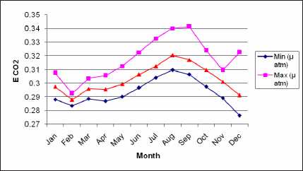
Figure 4 Distribution Monthly Data of CO₂ Exchange Coefficients between the Atmosphere and Ocean in 2007

In this study, the distribution of gas exchange coefficient obtained by the modified whitecap ^^OS/^^^^ data estimated from MODIS monthly data in 2007. The annual mean CO₂ gas exchange coefficient is 0.303 _m°^l m'2 _m0ath''μar_m- o^r 2.⁵2⁵ x IO'² (mol m ²month ¹μatm¹). This exchange coefficient corresponds Zhao (1995) result 5.7 x 10'² (mol m'²month'¹μatm'¹) (or 19.7 cm hour'¹) which is little smaller than 6.1x 10'² (mol m'²month'¹μatm'¹) (or 21cm hour'¹), which is global mean value of CO₂ estimated from C¹⁴ data (Broecker et al., 1986in Zhao,

1995). The seasonal variation can be seen clearly; especially the mean exchange coefficient varies much in May to October compared with November to April. Distributions of CO₂ exchange coefficients are shown in Figure 6 (d).

negative value; this indicates the flux into the ocean during the low SST in this month. Distributions of CO₂ flux are shown in Figure 6 (e).

Distribution Monthly Data of CO₂ Flux in 2007

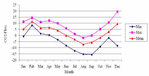
Figure 5 Distribution Monthly Data of CO₂ Flux in 2007

(a) Distribution of K CO2

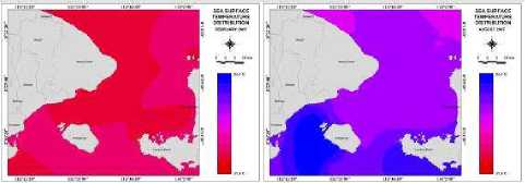
(b) Distribution of SST

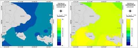
Figure 5 shows distribution monthly data of CO₂ flux between the atmosphere and ocean in 2007 from January until December, under the carbon dioxide flux value from -15.58 (mol m^² month’¹) to 19.45 (mol m’² month’¹). The lowest and highest transfer velocity of carbon dioxide could be seen on August and on February, with average CO₂ flux -7.14 (mol m’² month’¹) and 11.49 (mol m’² month’¹). The CO₂ flux which is determined from CO₂ transfer velocity (E) and △ p CO₂ becomes lower if SST, ' pC°∙ A^{the co}√^1ux ∙^ransf⅛^vel°^city "^e smaller. Result shows the negative CO₂ flux value indicates the flux into the ocean is from -7.14

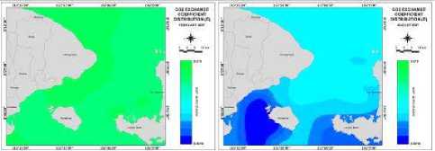
(c) Distribution of CO2 exchange coefficients

(mol m’² month’¹) on August to 11.49 (mol m’² month’¹) also on February. The positive CO₂ flux value indicates the flux into the atmosphere is from

(d) Distribution of pCO₂

0.44 mol m’² month’¹ on April to 19.45 mol m’² month’¹ on December. The following areas are strong sources for atmospheric CO₂ (positive Δ pCO2 values): i) the northwestern ofBadung Strait (due to

seasonal warming upwelling) and (ii) a few patchy areas near Lombok Barat regency (local upwelling).

(e) Distribution of CO₂ flux

Figure 6 (a, b, c, d, e) show the distributions variations ofKCO₂, SST, CO₂ exchange coefficients, “pCO₂, and CO₂ flux, respectively, in Badung and Lombok Straits variety in February and August

^{The avera}g^{e distributions o}f ^CO2 ^{flux in this month} become positive value; this indicates the flux into the atmosphere in this month. In August, the strong source areas include (i) the central Lombok Strait (upwelling) and (ii) the northern area ofLombok Strait temperate gyre (seasonal warming). The average ^{distributions o}f ^co2 ^fTux ^{in this month become}

• 4.    Conclusions and Sugestion
  
  Conclutions

. Within ALOS/FALSAR d._ta, the air-sea interaction at sea surface is determinate by directional wind wave and wind friction velocity from satellite-derived wind data which takes an important role for air sea interaction in the ocean.

^W“” ^alos∕^falsar data. th^eC⁰2 ^e≈ha^nge process between the atmosphere and the ocean at sea surface is determinate by carbon dioxide flux,

^{which is due to some factor}, ^{such as}: ∆p∞₂, E^co₂, SST, and total carbon acid.

^suges^tion. ,. .....

For the future study, it is recommended the deeper study using difference method on the calculation of the difference CO2 partial pressure between air and ocean, Δ pCO2, and on the calculation CO2 flux in ocean or in wider sea area with satellite and ground truth data.

References

Akiyama, M. 2002. “Air-Sea CO₂ Flux Estimation Using Satellite Data”. Proceeding of International Symposium on Remote Sensing. Tokai. Japan.

Feely. R.A., C.L. Sabine., T.Takahashi., and R.Wanninkhof. 2001. “Uptake and Storage of Carbon Dioxide in

„ ..^,heO“»U^?“^a.^lC?2^Su^                          i.U^SA-¹l^:1-⁴v . .

Frankignoulle, M., G. Abril.,A. Borges., I. Bourge., C. Canon., andB. Belille. 1998. Carbondioxide Emission fromEuropean Estuaries”. Science. 282: 434-436.

Hope, D., T. K. Kratz., and J. L. Riera. 1996. “ The Relationship Between Pco₂And Dissolved Organic Carbon In The Surface Waters Of27 Northern Wisconsin Lakes”. J. Environ. Qual. 19:1442-1445.

Keeling, C.D. 1995. Atmospheric Carbon Dioxide Concentrations from Mauna Loa Observatory Hawaii 1958^-1949 ^DroOl^CartettDMdeht^^           (CDl^C^TPAc^ve. „

Metzl,N.,A. Poisson., F. Louanchi., C. Brunet., B. Schauer., andB. Bres. 1995. SpatioTemporalDistributions .. . O^,A^⅛.^^^                                   -⁴7^:56;⁶⁹-.„ . ...

Meybeck, M.1993. Riverine Transport OfAtmospheric Carbon: Source, Global TypologyAnd Budget .

WceA.MJpoau.⁷⁰p⁴3-4⁶³         ..........„ „ „ .

Monahan, E.C. and M.C. Spillane. 1984. The Role of Oceanic Whitecaps in Air-Sea Gas Exchange.: Gas TransferofWaterSurface. Reidel Publishing Company.

Monahan, E.C. and K.W. David. 1989. “Comments OnVariations OfWhitecap Coverage WithWind Stress And Water Temperature”. T. Phys. Oceanography. 19: 706-709.

Schimel, D.S., J.I. House., and K.A. Hibbard. 2001. “RecentPatterns and Mechanisms ofCarbon Exchange „ . ^““'"Ec^^^            ........... „ . ...... .

Sugimori, Y andC.F. Zhao. 1995. TheCO₂ FluxEstimationintheNorthpacific OceanBasedon Satelliteand

Ship Data”. Proceeding of International Symposium on Remote Sensing. Taejon. Korea.

Suzuki,N.,N. Ebuchi., C.F. Zhao., I. Watabe., P. Shailesh., and Y. Sugimori. 2002. “Studyofthe Relationship between Non-Dimensional Roughness Length and wave Age Dependent on Fetch Effect”. Porsec.

. B^{alipoceedings}.2³5^-2⁴O

Takahashi.T., R.A. Feely., R.F. Weiss., R.H. Wanninkhof., D.W. Chipman., S.C. Sutherland., andT. Takahashi. 1997. “Global air-sea flux of CO₂: An Estimate Based On Measurements OfSea-Air pCO₂ Difference”. Proc. Natl. Acad. Sci. ColloquiumPaper. USA. 94: 8292-8299.

Toba, Y. and M. Chaen. 1973. Quantitative Expression cf the Breaking of the Wind Waves on the Sea Surface : Records of Oceanographic Works in Japan. Japan

Weiss, R.F. 1974. “Carbon Dioxide in Water and Seawater: the Solubility in water and Seawater”. Marine ... . ChT"?₂²:^203-2!⁵

Wu, J. 1988. Variations of Whitecap Coverage with Wind Stress and Water Temperature . J. Phys. Oceanography .18:1448-1453.

Zhao, C.F. 1995. The CO2 Flux Estimation in the North pacific Ocean Based on Satellite and Ship Data (Doctor Dissertation>. Doctor Program in Center ofEnvironment Remote Sensing. Chiba University, Japan.

158